suppressPackageStartupMessages({
  library(multcomp)
  library(car)
  library(tidyr)
  library(lme4)
  library(ggplot2)
  library(ggtext)
  library(ggpmisc)
  library(nlme)
  library(latex2exp)
  library(kableExtra)
  library(broom)
  library(dplyr)
  library(MuMIn)
})

options(warn = -1)
RES <- readRDS("~/Documents/Master Thesis/Master-Thesis-P-kinetics/data/RES.rds")
D <- RES$D2
d <- RES$dataIn [1]:
Model Agroscope \[Y_{rel}\sim A*(1-e^{rate*P_{CO_2}+Env})\]
Wir ersetzen nur rate mit unserer Schätzung k: \[Y_{rel}\sim A*(1-e^{k*P_{CO_2}+Env})\]
Sind unsere Modelparameter gute Prediktoren?? \[Y_{rel}\sim A*(1-e^{k*PS+Env} )\]
Es gibt noch die Kovariaten Niederschlag pro Jahr, Jahresdurchschnittstemperatur und Temperatur in Jugendphase
In [2]:
library(GGally)

ggpairs(D,
  aes(col=Site, shape = Treatment,alpha = 0.6),
  columns = c("soil_0_20_P_AAE10", "soil_0_20_P_CO2", "PS", "k", "kPS"),
  lower = list(continuous = wrap("points", size = 1.3)),
  upper = list(continuous = "blank", combo = "blank", discrete = "blank"))  # Adjust size here


p6 <- ggplot(D,aes(y=soil_0_20_P_AAE10, x=soil_0_20_P_CO2, col=Site, size = Treatment)) +
  geom_point(shape = 7) +
  scale_x_log10() + scale_y_log10() +
  labs(x=TeX("$P_{H_2O10}(mg/kg Soil)$"),
         y=TeX("$P_{AAEDTA}(mg/kg Soil)$")); p6

p7 <- ggplot(D,aes(y=PS, x=soil_0_20_P_CO2, col=Site, size = Treatment)) +
  geom_point(shape = 7) +
  scale_x_log10() + scale_y_log10() +
  labs(x=TeX("$P_{CO_2}(mg/kg Soil)$"),
          y=TeX("$PS(mg/kg Soil)$")); p7

p8 <- ggplot(D,aes(y=k, x=soil_0_20_P_CO2, col=Site, size = Treatment)) +
  geom_point(shape = 7) +
  scale_x_log10() +
  labs(x=TeX("$P_{CO_2}(mg/kg Soil)$"),
         y=TeX("$k(1/s)$")); p8

p9 <- ggplot(D,aes(y=k*PS, x=soil_0_20_P_CO2, col=Site, size = Treatment)) +
  geom_point(shape = 7) +
  scale_x_log10() + scale_y_log10() +
  labs(x=TeX("$P_{CO_2}(mg/kg Soil)$"),
         y=TeX("$v=k*PS(mg/s*kg Soil)$"));p9


p11 <- ggplot(D,aes(y=PS, x=soil_0_20_P_AAE10, col=Site, size = Treatment)) +
  scale_x_log10() + scale_y_log10() +
  geom_point(shape = 7) +
  labs(x=TeX("$P_{AAEDTA}(mg/kg Soil)$"),
         y=TeX("$PS(mg/kg Soil)$")); p11

p12 <- ggplot(D,aes(y=k, x=soil_0_20_P_AAE10, col=Site, size = Treatment)) +
  geom_point(shape = 7) +
   scale_x_log10() + scale_y_log10() +
  labs(x=TeX("$P_{AAEDTA}(mg/kg Soil)$"),
         y=TeX("$k(1/s)$"))

p12

p13 <- ggplot(D,aes(y=k*PS, x=soil_0_20_P_AAE10, col=Site, size = Treatment)) +
  scale_x_log10() + scale_y_log10() +
  geom_point(shape = 7) +
  labs(x=TeX("$P_{AAEDTA}(mg/kg Soil)$"),
         y=TeX("$log(v)=log(k*PS)(mg/s*kg Soil)$"))

p13
Nun noch die Linearen Regressionen, die ausstehend sind:
(1|year) + (1|Site) + (1|Site:block) + (Treatment|Site)
Random intercept per year and site, block nested in site. and Treatment nested in site (could also be modelled as a random slope to allow for correlations)
wir sind abe nicht an einem Treatment effekt interesseiert. drum verwerfen wir Treatment als Random UND Fixed effekt.
- Vergleiche PS, k und kPS mit
In [3]:
# Wovon hängen Modelparameter ab?

library(lmerTest)
Attaching package: 'lmerTest'The following object is masked from 'package:lme4':
lmerThe following object is masked from 'package:stats':
stepfit.soil.PS <- lmer(log(PS) ~ soil_0_20_clay+ soil_0_20_pH_H2O + soil_0_20_Corg + soil_0_20_silt + Feox + Alox + (1|year) + (1|Site) + (1|Site:block) + (1|Site:Treatment), D)boundary (singular) fit: see help('isSingular')# fit.soil.PS2 <- lmer(log(PS) ~ soil_0_20_clay+ soil_0_20_pH_H2O + soil_0_20_Corg + soil_0_20_silt + (1|year) + (1|Site) + (1|Site:block) + (1|Site:Treatment), D)
fit.soil.k <- lmer(k ~ soil_0_20_clay+ soil_0_20_pH_H2O + soil_0_20_Corg + soil_0_20_silt + Feox + Alox + (1|year) + (1|Site) + (1|Site:block) + (1|Site:Treatment), D)boundary (singular) fit: see help('isSingular')fit.soil.kPS <- lmer(I(log(k*PS))~ soil_0_20_clay+ soil_0_20_pH_H2O + soil_0_20_Corg + soil_0_20_silt + Feox + Alox + (1|year) + (1|Site) + (1|Site:block) + (1|Site:Treatment), D)boundary (singular) fit: see help('isSingular')fit.soil.kPS2<- lmer(I(k*log(PS))~ soil_0_20_clay+ soil_0_20_pH_H2O + soil_0_20_Corg + soil_0_20_silt + Feox + Alox + (1|year) + (1|Site) + (1|Site:block) + (1|Site:Treatment), D)boundary (singular) fit: see help('isSingular')fit.soil.CO2 <- lmer(log(soil_0_20_P_CO2)~ soil_0_20_clay+ soil_0_20_pH_H2O + soil_0_20_Corg + soil_0_20_silt + Feox + Alox + (1|year) + (1|Site) + (1|Site:block) + (1|Site:Treatment), D)boundary (singular) fit: see help('isSingular')fit.soil.AAE10<-lmer(log(soil_0_20_P_AAE10)~ soil_0_20_clay+ soil_0_20_pH_H2O + soil_0_20_Corg + soil_0_20_silt + Feox + Alox + (1|year) + (1|Site) + (1|Site:block) + (1|Site:Treatment), D)
r.squaredGLMM(fit.soil.kPS) R2m R2c
[1,] 0.06987647 0.9104987r.squaredGLMM(fit.soil.kPS2) R2m R2c
[1,] 0.3680394 0.8251728fit.kin.Yrel <- lmer(Ymain_rel ~ k * log(PS) + (1|year) + (1|Site) + (1|Site:block), D)boundary (singular) fit: see help('isSingular')fit.kin.Ynorm <- lmer(Ymain_norm ~ k + log(PS) + (1|year) + (1|Site) + (1|Site:block), D, subset = Treatment != "P166")boundary (singular) fit: see help('isSingular')r.squaredGLMM(fit.kin.Ynorm) R2m R2c
[1,] 0.01132987 0.3222732fit.kin.Ynorm <- lmer(Ymain_norm ~ k * log(PS) + (1|year) + (1|Site) + (1|Site:block), D, subset = Treatment != "P166")boundary (singular) fit: see help('isSingular')r.squaredGLMM(fit.kin.Ynorm) R2m R2c
[1,] 0.01389348 0.3206529fit.kin.Ynorm <- lmer(Ymain_norm ~ k * log(PS) + (1|year), D, subset = Treatment != "P166")
r.squaredGLMM(fit.kin.Ynorm) R2m R2c
[1,] 0.03949443 0.2327285fit.kin.Ynorm <- lmer(Ymain_norm ~ k * log(PS) + (1|year) + (1|Site) + (1|Site:block), D)boundary (singular) fit: see help('isSingular')r.squaredGLMM(fit.kin.Ynorm) R2m R2c
[1,] 0.02354704 0.220675fit.kin.Ynorm <- lmer(Ymain_norm ~ k * log(PS) + (1|year) + (1|Site) + (1|Site:block), D, subset = Treatment == "P0")boundary (singular) fit: see help('isSingular')r.squaredGLMM(fit.kin.Ynorm) R2m R2c
[1,] 0.02559532 0.4046309summary(fit.kin.Ynorm, ddf="Kenward-Roger")Linear mixed model fit by REML. t-tests use Kenward-Roger's method [
lmerModLmerTest]
Formula: Ymain_norm ~ k * log(PS) + (1 | year) + (1 | Site) + (1 | Site:block)
Data: D
Subset: Treatment == "P0"
REML criterion at convergence: 237
Scaled residuals:
Min 1Q Median 3Q Max
-2.2274 -0.2703 0.0472 0.3082 4.2211
Random effects:
Groups Name Variance Std.Dev.
Site:block (Intercept) 0.00000 0.0000
year (Intercept) 0.09912 0.3148
Site (Intercept) 0.08030 0.2834
Residual 0.28181 0.5309
Number of obs: 140, groups: Site:block, 20; year, 7; Site, 5
Fixed effects:
Estimate Std. Error df t value Pr(>|t|)
(Intercept) 2.1092 1.8704 13.9709 1.128 0.278
k -3.5406 10.2424 13.6015 -0.346 0.735
log(PS) 0.2281 0.5500 13.3627 0.415 0.685
k:log(PS) -0.5902 3.0029 13.2694 -0.197 0.847
Correlation of Fixed Effects:
(Intr) k lg(PS)
k -0.947
log(PS) 0.986 -0.943
k:log(PS) -0.936 0.992 -0.948
optimizer (nloptwrap) convergence code: 0 (OK)
boundary (singular) fit: see help('isSingular')fit.kin.Ynorm <- lmer(Ymain_norm ~ k * log(PS) + (1|year) + (1|Site) + (1|Site:block), D, subset = Treatment == "P100")
r.squaredGLMM(fit.kin.Ynorm) R2m R2c
[1,] 0.03216247 0.2739785fit.grud.CO2.Ynorm <- lmer(Ymain_norm ~ log(soil_0_20_P_CO2) + (1|year) + (1|Site) + (1|Site:block), D, subset = Treatment != "P166")
r.squaredGLMM(fit.grud.CO2.Ynorm) R2m R2c
[1,] 0.226324 0.4317041fit.grud.AAE10.Ynorm <- lmer(Ymain_norm ~ log(soil_0_20_P_AAE10) + (1|year) + (1|Site) + (1|Site:block), D, subset = Treatment != "P166")
r.squaredGLMM(fit.grud.AAE10.Ynorm) R2m R2c
[1,] 0.202547 0.4445619fit.grud.CO2.AAE10.Ynorm <- lmer(Ymain_norm ~ log(soil_0_20_P_CO2) * log(soil_0_20_P_AAE10) + (1|year) + (1|Site) + (1|Site:block), D, subset = Treatment != "P166")
r.squaredGLMM(fit.grud.CO2.AAE10.Ynorm) R2m R2c
[1,] 0.2239347 0.4394869# compare with k*log(PS)
fit.kin.Ynorm <- lmer(Ymain_norm ~ k*log(PS) + (1|year) + (1|Site) + (1|Site:block), D, subset = Treatment != "P166")boundary (singular) fit: see help('isSingular')r.squaredGLMM(fit.kin.Ynorm) R2m R2c
[1,] 0.01389348 0.3206529fit.kin.Ynorm <- lmer(Ymain_norm ~ k * log(PS) + (1|year) + (1|Site) + (1|Site:block), D, subset = Treatment != "P166")boundary (singular) fit: see help('isSingular')fit.kin.Pexport <- lmer(annual_P_uptake ~ k * log(PS) + (1|year) + (1|Site) + (1|Site:block), D)boundary (singular) fit: see help('isSingular')fit.kin.Pbalance <- lmer(annual_P_balance ~ k * log(PS) + (1|year) + (1|Site) + (1|Site:block), D)
car::vif(lm(Ymain_norm ~ (k) * log(PS) + crop, D))there are higher-order terms (interactions) in this model
consider setting type = 'predictor'; see ?vif GVIF Df GVIF^(1/(2*Df))
k 12.721081 1 3.566662
log(PS) 12.182601 1 3.490358
crop 1.044188 5 1.004333
k:log(PS) 29.426189 1 5.424591car::vif(lm(Ymain_norm ~ scale(k) * scale(log(PS)) + crop, D))there are higher-order terms (interactions) in this model
consider setting type = 'predictor'; see ?vif GVIF Df GVIF^(1/(2*Df))
scale(k) 1.120802 1 1.058679
scale(log(PS)) 1.071093 1 1.034936
crop 1.044188 5 1.004333
scale(k):scale(log(PS)) 1.015027 1 1.007486car::vif(lm(Ymain_norm ~ k + log(PS) + crop, D)) GVIF Df GVIF^(1/(2*Df))
k 1.112232 1 1.054624
log(PS) 1.068219 1 1.033547
crop 1.043502 5 1.004267car::vif(lm(Ymain_norm ~ I(k * (PS)) + k + log(PS) + crop, D)) GVIF Df GVIF^(1/(2*Df))
I(k * (PS)) 4.640782 1 2.154247
k 2.041541 1 1.428825
log(PS) 4.690858 1 2.165839
crop 1.045520 5 1.004461with(D, hist(I(exp(k) * (PS))))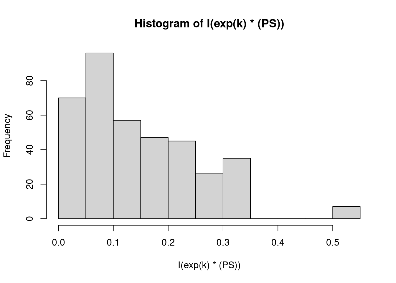
with(D, hist(log(PS)))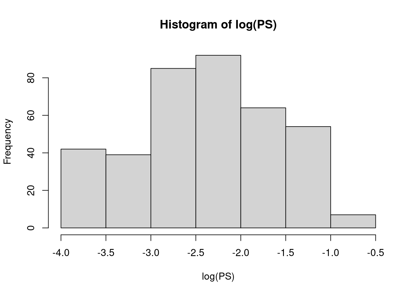
r.squaredGLMM(fit.kin.Ynorm) R2m R2c
[1,] 0.01389348 0.3206529anova(fit.soil.PS)Type III Analysis of Variance Table with Satterthwaite's method
Sum Sq Mean Sq NumDF DenDF F value Pr(>F)
soil_0_20_clay 0.002083 0.002083 1 38.033 0.0569 0.81272
soil_0_20_pH_H2O 0.000134 0.000134 1 37.384 0.0037 0.95203
soil_0_20_Corg 0.161222 0.161222 1 31.905 4.4045 0.04385 *
soil_0_20_silt 0.004846 0.004846 1 38.673 0.1324 0.71793
Feox 0.001149 0.001149 1 0.347 0.0314 0.91632
Alox 0.012358 0.012358 1 0.257 0.3376 0.79220
---
Signif. codes: 0 '***' 0.001 '**' 0.01 '*' 0.05 '.' 0.1 ' ' 1summary(glht(fit.soil.PS))
     Simultaneous Tests for General Linear Hypotheses

Fit: lmer(formula = log(PS) ~ soil_0_20_clay + soil_0_20_pH_H2O +
    soil_0_20_Corg + soil_0_20_silt + Feox + Alox + (1 | year) +
    (1 | Site) + (1 | Site:block) + (1 | Site:Treatment), data = D)

Linear Hypotheses:
                       Estimate Std. Error z value Pr(>|z|)
(Intercept) == 0      -4.315984   2.026178  -2.130    0.175
soil_0_20_clay == 0   -0.007322   0.030690  -0.239    1.000
soil_0_20_pH_H2O == 0 -0.007820   0.129130  -0.061    1.000
soil_0_20_Corg == 0    0.635270   0.302698   2.099    0.189
soil_0_20_silt == 0   -0.010244   0.028153  -0.364    0.999
Feox == 0             -0.052865   0.298418  -0.177    1.000
Alox == 0              0.603465   1.038573   0.581    0.989
(Adjusted p values reported -- single-step method)
# Fazit: PS wird von treatment stark beeinfluss, k eher nicht (dafür von site)
anova(fit.soil.k)Type III Analysis of Variance Table with Satterthwaite's method
Sum Sq Mean Sq NumDF DenDF F value Pr(>F)
soil_0_20_clay 0.0118462 0.0118462 1 39.973 10.7210 0.002191 **
soil_0_20_pH_H2O 0.0011812 0.0011812 1 38.291 1.0690 0.307665
soil_0_20_Corg 0.0090425 0.0090425 1 35.487 8.1836 0.007040 **
soil_0_20_silt 0.0012705 0.0012705 1 10.804 1.1498 0.306956
Feox 0.0000004 0.0000004 1 0.968 0.0003 0.988186
Alox 0.0004765 0.0004765 1 1.117 0.4312 0.620552
---
Signif. codes: 0 '***' 0.001 '**' 0.01 '*' 0.05 '.' 0.1 ' ' 1summary(glht(fit.soil.k))
     Simultaneous Tests for General Linear Hypotheses

Fit: lmer(formula = k ~ soil_0_20_clay + soil_0_20_pH_H2O + soil_0_20_Corg +
    soil_0_20_silt + Feox + Alox + (1 | year) + (1 | Site) +
    (1 | Site:block) + (1 | Site:Treatment), data = D)

Linear Hypotheses:
                       Estimate Std. Error z value Pr(>|z|)
(Intercept) == 0       0.608404   0.351212   1.732  0.37844
soil_0_20_clay == 0   -0.016659   0.005088  -3.274  0.00683 **
soil_0_20_pH_H2O == 0 -0.022256   0.021526  -1.034  0.84750
soil_0_20_Corg == 0    0.137353   0.048014   2.861  0.02612 *
soil_0_20_silt == 0    0.004094   0.003818   1.072  0.82673
Feox == 0              0.001024   0.054815   0.019  1.00000
Alox == 0             -0.128860   0.196235  -0.657  0.97804
---
Signif. codes:  0 '***' 0.001 '**' 0.01 '*' 0.05 '.' 0.1 ' ' 1
(Adjusted p values reported -- single-step method)anova(fit.soil.kPS)Type III Analysis of Variance Table with Satterthwaite's method
Sum Sq Mean Sq NumDF DenDF F value Pr(>F)
soil_0_20_clay 0.27383 0.27383 1 37.930 3.2642 0.078745 .
soil_0_20_pH_H2O 0.00989 0.00989 1 37.703 0.1179 0.733211
soil_0_20_Corg 0.63137 0.63137 1 32.625 7.5263 0.009799 **
soil_0_20_silt 0.00591 0.00591 1 39.206 0.0705 0.791988
Feox 0.04311 0.04311 1 0.225 0.5139 0.775407
Alox 0.00881 0.00881 1 0.130 0.1050 0.904677
---
Signif. codes: 0 '***' 0.001 '**' 0.01 '*' 0.05 '.' 0.1 ' ' 1summary(glht(fit.soil.kPS))
     Simultaneous Tests for General Linear Hypotheses

Fit: lmer(formula = I(log(k * PS)) ~ soil_0_20_clay + soil_0_20_pH_H2O +
    soil_0_20_Corg + soil_0_20_silt + Feox + Alox + (1 | year) +
    (1 | Site) + (1 | Site:block) + (1 | Site:Treatment), data = D)

Linear Hypotheses:
                      Estimate Std. Error z value Pr(>|z|)
(Intercept) == 0      -5.22214    2.67612  -1.951   0.2528
soil_0_20_clay == 0   -0.08506    0.04708  -1.807   0.3311
soil_0_20_pH_H2O == 0 -0.06836    0.19908  -0.343   0.9993
soil_0_20_Corg == 0    1.29047    0.47039   2.743   0.0372 *
soil_0_20_silt == 0   -0.01141    0.04296  -0.266   0.9998
Feox == 0              0.24813    0.34612   0.717   0.9669
Alox == 0              0.36766    1.13436   0.324   0.9995
---
Signif. codes:  0 '***' 0.001 '**' 0.01 '*' 0.05 '.' 0.1 ' ' 1
(Adjusted p values reported -- single-step method)anova(fit.kin.Yrel)Type III Analysis of Variance Table with Satterthwaite's method
Sum Sq Mean Sq NumDF DenDF F value Pr(>F)
k 7760.6 7760.6 1 301.92 5.7850 0.01676 *
log(PS) 5373.3 5373.3 1 302.30 4.0054 0.04625 *
k:log(PS) 8701.9 8701.9 1 302.51 6.4866 0.01136 *
---
Signif. codes: 0 '***' 0.001 '**' 0.01 '*' 0.05 '.' 0.1 ' ' 1anova(fit.kin.Ynorm)Type III Analysis of Variance Table with Satterthwaite's method
Sum Sq Mean Sq NumDF DenDF F value Pr(>F)
k 0.151218 0.151218 1 269.22 0.6379 0.4252
log(PS) 0.019202 0.019202 1 268.74 0.0810 0.7762
k:log(PS) 0.201373 0.201373 1 268.71 0.8494 0.3575anova(fit.kin.Pexport)Type III Analysis of Variance Table with Satterthwaite's method
Sum Sq Mean Sq NumDF DenDF F value Pr(>F)
k 45.672 45.672 1 294.59 0.5847 0.4451
log(PS) 84.870 84.870 1 295.00 1.0866 0.2981
k:log(PS) 50.311 50.311 1 295.03 0.6441 0.4229anova(fit.soil.CO2)Type III Analysis of Variance Table with Satterthwaite's method
Sum Sq Mean Sq NumDF DenDF F value Pr(>F)
soil_0_20_clay 0.017260 0.017260 1 38.410 0.1191 0.7319
soil_0_20_pH_H2O 0.080631 0.080631 1 38.254 0.5562 0.4604
soil_0_20_Corg 0.029198 0.029198 1 38.466 0.2014 0.6561
soil_0_20_silt 0.005041 0.005041 1 40.886 0.0348 0.8530
Feox 0.102556 0.102556 1 14.728 0.7074 0.4138
Alox 0.001448 0.001448 1 4.877 0.0100 0.9244anova(fit.soil.AAE10)Type III Analysis of Variance Table with Satterthwaite's method
Sum Sq Mean Sq NumDF DenDF F value Pr(>F)
soil_0_20_clay 0.000000 0.000000 1 34.138 0.0000 0.9993
soil_0_20_pH_H2O 0.022655 0.022655 1 30.975 0.3822 0.5409
soil_0_20_Corg 0.091344 0.091344 1 27.873 1.5412 0.2248
soil_0_20_silt 0.033276 0.033276 1 34.322 0.5614 0.4588
Feox 0.023984 0.023984 1 7.835 0.4047 0.5428
Alox 0.104053 0.104053 1 3.886 1.7556 0.2577anova(fit.kin.Pbalance)Type III Analysis of Variance Table with Satterthwaite's method
Sum Sq Mean Sq NumDF DenDF F value Pr(>F)
k 124.7 124.7 1 275.62 0.6004 0.4391
log(PS) 4906.5 4906.5 1 285.15 23.6264 1.935e-06 ***
k:log(PS) 120.8 120.8 1 280.10 0.5819 0.4462
---
Signif. codes: 0 '***' 0.001 '**' 0.01 '*' 0.05 '.' 0.1 ' ' 1summary(fit.kin.Pbalance)Linear mixed model fit by REML. t-tests use Satterthwaite's method [
lmerModLmerTest]
Formula: annual_P_balance ~ k * log(PS) + (1 | year) + (1 | Site) + (1 |
Site:block)
Data: D
REML criterion at convergence: 2719.8
Scaled residuals:
Min 1Q Median 3Q Max
-4.3960 -0.5775 0.0036 0.5915 2.8874
Random effects:
Groups Name Variance Std.Dev.
Site:block (Intercept) 27.20 5.216
year (Intercept) 54.22 7.363
Site (Intercept) 127.50 11.292
Residual 207.67 14.411
Number of obs: 330, groups: Site:block, 20; year, 7; Site, 5
Fixed effects:
Estimate Std. Error df t value Pr(>|t|)
(Intercept) 59.223 11.538 62.390 5.133 3.02e-06 ***
k 42.436 54.765 275.615 0.775 0.439
log(PS) 21.577 4.439 285.149 4.861 1.93e-06 ***
k:log(PS) 17.933 23.508 280.101 0.763 0.446
---
Signif. codes: 0 '***' 0.001 '**' 0.01 '*' 0.05 '.' 0.1 ' ' 1
Correlation of Fixed Effects:
(Intr) k lg(PS)
k -0.827
log(PS) 0.807 -0.897
k:log(PS) -0.792 0.941 -0.970fit.kin.Pbalance |> r.squaredGLMM() R2m R2c
[1,] 0.4896394 0.7455866fit.kin.Pexport |> r.squaredGLMM() R2m R2c
[1,] 0.04012948 0.7758557fit.kin.Yrel |> r.squaredGLMM() R2m R2c
[1,] 0.01503741 0.5119295fit.kin.Ynorm |> r.squaredGLMM() R2m R2c
[1,] 0.01389348 0.3206529# Verhalten der Modelparameter und Ertragsdaten auf P-CO2 und P-AAE10Since we now model two measurement methods, we do not expect correlations by Site/year/etc
In [4]:
# fit.PS       <- lm(PS            ~ soil_0_20_P_CO2 + soil_0_20_P_AAE10, D)
fit.grud.PS       <- lm(log(PS)         ~ log(soil_0_20_P_CO2) + log(soil_0_20_P_AAE10), D)
fit.grud.k        <- lm(k               ~ log(soil_0_20_P_CO2) + log(soil_0_20_P_AAE10), D)
fit.grud.kPS      <- lm(I(log(k*PS))    ~ log(soil_0_20_P_CO2) + log(soil_0_20_P_AAE10), D)

fit.grud.CO2.Yrel     <- lmer(Ymain_rel       ~ log(soil_0_20_P_CO2) + (1|year) + (1|Site)  + (1|Site:block) + (1|Site:Treatment), D)
fit.grud.AAE10.Yrel     <- lmer(Ymain_rel       ~ log(soil_0_20_P_AAE10) + (1|year) + (1|Site)  + (1|Site:block) + (1|Site:Treatment), D)
fit.grud.Yrel     <- lmer(Ymain_rel       ~ log(soil_0_20_P_CO2) * log(soil_0_20_P_AAE10) + (1|year) + (1|Site)  + (1|Site:block) + (1|Site:Treatment), D)


# this is hopeless, since cannot log becaus of 0's
fit.CO2.Pexport     <- lmer(annual_P_uptake     ~ log(soil_0_20_P_CO2) + (1|year) + (1|Site)  + (1|Site:block) + (1|Site:Treatment), D)
boundary (singular) fit: see help('isSingular')fit.AAE10.Pexport <- lmer(annual_P_uptake ~ log(soil_0_20_P_AAE10) + (1|year) + (1|Site) + (1|Site:block) + (1|Site:Treatment), D)boundary (singular) fit: see help('isSingular')fit.grud.Pexport <- lmer(annual_P_uptake ~ log(soil_0_20_P_CO2) * log(soil_0_20_P_AAE10) + (1|year) + (1|Site) + (1|Site:block) + (1|Site:Treatment), D)boundary (singular) fit: see help('isSingular')fit.CO2.Pbalance <- lmer(annual_P_balance ~ log(soil_0_20_P_CO2) + (1|year) + (1|Site) + (1|Site:block) + (1|Site:Treatment), D)boundary (singular) fit: see help('isSingular')fit.AAE10.Pbalance <- lmer(annual_P_balance ~ log(soil_0_20_P_AAE10) + (1|year) + (1|Site) + (1|Site:block) + (1|Site:Treatment), D)boundary (singular) fit: see help('isSingular')fit.grud.Pbalance <- lmer(annual_P_balance ~ log(soil_0_20_P_CO2) * log(soil_0_20_P_AAE10) + (1|year) + (1|Site) + (1|Site:block) + (1|Site:Treatment), D)boundary (singular) fit: see help('isSingular')#summary(glht(fit.PS))
# Fazit: PS wird von treatment stark beeinfluss, k eher nicht (dafür von site)
summary(glht(fit.grud.PS))
     Simultaneous Tests for General Linear Hypotheses

Fit: lm(formula = log(PS) ~ log(soil_0_20_P_CO2) + log(soil_0_20_P_AAE10),
    data = D)

Linear Hypotheses:
                            Estimate Std. Error t value Pr(>|t|)
(Intercept) == 0            -1.62462    0.23590  -6.887   <1e-05 ***
log(soil_0_20_P_CO2) == 0    1.03597    0.06088  17.017   <1e-05 ***
log(soil_0_20_P_AAE10) == 0 -0.01187    0.06067  -0.196    0.966
---
Signif. codes:  0 '***' 0.001 '**' 0.01 '*' 0.05 '.' 0.1 ' ' 1
(Adjusted p values reported -- single-step method)summary(glht(fit.grud.k))
     Simultaneous Tests for General Linear Hypotheses

Fit: lm(formula = k ~ log(soil_0_20_P_CO2) + log(soil_0_20_P_AAE10),
    data = D)

Linear Hypotheses:
                             Estimate Std. Error t value Pr(>|t|)
(Intercept) == 0             0.101007   0.029593   3.413  0.00148 **
log(soil_0_20_P_CO2) == 0   -0.027290   0.007637  -3.573  < 0.001 ***
log(soil_0_20_P_AAE10) == 0  0.021789   0.007612   2.863  0.00724 **
---
Signif. codes:  0 '***' 0.001 '**' 0.01 '*' 0.05 '.' 0.1 ' ' 1
(Adjusted p values reported -- single-step method)summary(glht(fit.grud.kPS))
     Simultaneous Tests for General Linear Hypotheses

Fit: lm(formula = I(log(k * PS)) ~ log(soil_0_20_P_CO2) + log(soil_0_20_P_AAE10),
    data = D)

Linear Hypotheses:
                            Estimate Std. Error t value Pr(>|t|)
(Intercept) == 0            -3.67498    0.24189 -15.193   <0.001 ***
log(soil_0_20_P_CO2) == 0    0.91106    0.06243  14.594   <0.001 ***
log(soil_0_20_P_AAE10) == 0  0.06769    0.06222   1.088    0.391
---
Signif. codes:  0 '***' 0.001 '**' 0.01 '*' 0.05 '.' 0.1 ' ' 1
(Adjusted p values reported -- single-step method)summary(fit.grud.Yrel)Linear mixed model fit by REML. t-tests use Satterthwaite's method [
lmerModLmerTest]
Formula: Ymain_rel ~ log(soil_0_20_P_CO2) * log(soil_0_20_P_AAE10) + (1 |
year) + (1 | Site) + (1 | Site:block) + (1 | Site:Treatment)
Data: D
REML criterion at convergence: 1731.6
Scaled residuals:
Min 1Q Median 3Q Max
-3.0471 -0.6233 -0.0496 0.5860 3.1830
Random effects:
Groups Name Variance Std.Dev.
Site:block (Intercept) 4.449 2.109
Site:Treatment (Intercept) 29.254 5.409
year (Intercept) 169.205 13.008
Site (Intercept) 15.292 3.911
Residual 191.096 13.824
Number of obs: 212, groups:
Site:block, 16; Site:Treatment, 12; year, 5; Site, 4
Fixed effects:
Estimate Std. Error df t value
(Intercept) 86.797 20.421 86.613 4.250
log(soil_0_20_P_CO2) 17.430 11.945 164.224 1.459
log(soil_0_20_P_AAE10) 4.593 5.056 95.253 0.909
log(soil_0_20_P_CO2):log(soil_0_20_P_AAE10) -4.372 3.066 148.783 -1.426
Pr(>|t|)
(Intercept) 5.36e-05 ***
log(soil_0_20_P_CO2) 0.146
log(soil_0_20_P_AAE10) 0.366
log(soil_0_20_P_CO2):log(soil_0_20_P_AAE10) 0.156
---
Signif. codes: 0 '***' 0.001 '**' 0.01 '*' 0.05 '.' 0.1 ' ' 1
Correlation of Fixed Effects:
(Intr) lg(_0_20_P_CO2) l(_0_20_P_A
lg(_0_20_P_CO2) 0.765
l(_0_20_P_A -0.946 -0.786
l(_0_20_P_CO2): -0.605 -0.950 0.630 summary(fit.grud.Pexport)Linear mixed model fit by REML. t-tests use Satterthwaite's method [
lmerModLmerTest]
Formula: annual_P_uptake ~ log(soil_0_20_P_CO2) * log(soil_0_20_P_AAE10) +
(1 | year) + (1 | Site) + (1 | Site:block) + (1 | Site:Treatment)
Data: D
REML criterion at convergence: 1834.1
Scaled residuals:
Min 1Q Median 3Q Max
-3.2817 -0.4518 -0.0801 0.4504 4.7520
Random effects:
Groups Name Variance Std.Dev.
Site:block (Intercept) 0.00 0.000
Site:Treatment (Intercept) 0.00 0.000
year (Intercept) 75.76 8.704
Site (Intercept) 30.12 5.489
Residual 64.95 8.059
Number of obs: 259, groups:
Site:block, 16; Site:Treatment, 12; year, 6; Site, 4
Fixed effects:
Estimate Std. Error df
(Intercept) 30.6288 11.3421 133.4332
log(soil_0_20_P_CO2) 9.8213 5.8400 250.2829
log(soil_0_20_P_AAE10) -0.8099 2.7078 240.1731
log(soil_0_20_P_CO2):log(soil_0_20_P_AAE10) -1.1650 1.4145 250.3524
t value Pr(>|t|)
(Intercept) 2.700 0.00782 **
log(soil_0_20_P_CO2) 1.682 0.09387 .
log(soil_0_20_P_AAE10) -0.299 0.76511
log(soil_0_20_P_CO2):log(soil_0_20_P_AAE10) -0.824 0.41095
---
Signif. codes: 0 '***' 0.001 '**' 0.01 '*' 0.05 '.' 0.1 ' ' 1
Correlation of Fixed Effects:
(Intr) lg(_0_20_P_CO2) l(_0_20_P_A
lg(_0_20_P_CO2) 0.786
l(_0_20_P_A -0.916 -0.847
l(_0_20_P_CO2): -0.624 -0.951 0.675
optimizer (nloptwrap) convergence code: 0 (OK)
boundary (singular) fit: see help('isSingular')summary(fit.grud.Pbalance)Linear mixed model fit by REML. t-tests use Satterthwaite's method [
lmerModLmerTest]
Formula: annual_P_balance ~ log(soil_0_20_P_CO2) * log(soil_0_20_P_AAE10) +
(1 | year) + (1 | Site) + (1 | Site:block) + (1 | Site:Treatment)
Data: D
REML criterion at convergence: 2121.6
Scaled residuals:
Min 1Q Median 3Q Max
-4.3603 -0.5255 0.0342 0.5431 2.8598
Random effects:
Groups Name Variance Std.Dev.
Site:block (Intercept) 0.000e+00 0.000000
Site:Treatment (Intercept) 5.170e+02 22.737367
year (Intercept) 6.267e+01 7.916138
Site (Intercept) 1.570e-06 0.001253
Residual 1.118e+02 10.571431
Number of obs: 274, groups:
Site:block, 16; Site:Treatment, 12; year, 6; Site, 4
Fixed effects:
Estimate Std. Error df t value
(Intercept) -5.502 15.689 163.186 -0.351
log(soil_0_20_P_CO2) -10.403 8.497 258.394 -1.224
log(soil_0_20_P_AAE10) 1.981 3.669 262.994 0.540
log(soil_0_20_P_CO2):log(soil_0_20_P_AAE10) 1.417 2.231 258.328 0.635
Pr(>|t|)
(Intercept) 0.726
log(soil_0_20_P_CO2) 0.222
log(soil_0_20_P_AAE10) 0.590
log(soil_0_20_P_CO2):log(soil_0_20_P_AAE10) 0.526
Correlation of Fixed Effects:
(Intr) lg(_0_20_P_CO2) l(_0_20_P_A
lg(_0_20_P_CO2) 0.655
l(_0_20_P_A -0.879 -0.706
l(_0_20_P_CO2): -0.491 -0.937 0.541
optimizer (nloptwrap) convergence code: 0 (OK)
boundary (singular) fit: see help('isSingular')fit.grud.Pbalance |> r.squaredGLMM() R2m R2c
[1,] 0.01324864 0.8405073fit.grud.Pexport |> r.squaredGLMM() R2m R2c
[1,] 0.07722235 0.6491677fit.grud.Yrel |> r.squaredGLMM() R2m R2c
[1,] 0.09927847 0.5794631save.image(file = "~/Documents/Master Thesis/Master-Thesis-P-kinetics/data/results_coefficient_analysis")In [5]:
create_coef_table <- function(lmer_models,
                              covariate_order = NULL,
                              covariate_labels = NULL, # NEU: Benannter Vektor für Zeilennamen
                              model_labels = NULL) {   # NEU: Benannter Vektor für Spaltennamen

  # Extract coefficients and p-values (Ihre Originalfunktion, keine Änderung hier)
  extract_coef_info <- function(model) {
    # ... (keine Änderung, Ihr Code bleibt hier)
    coef_matrix <- summary(model)|> coef()
    estimates <- coef_matrix[, 1]
    p_values <- coef_matrix[, ncol(coef_matrix)]
    formatted_coef <- sapply(seq_along(estimates), function(i) {
      est_str <- sprintf("%.3f", estimates[i])
      stars <- if (p_values[i] < 0.001) "***" else
               if (p_values[i] < 0.01) "** " else
               if (p_values[i] < 0.05) "* " else  ""
      paste0(stars, est_str)
    })
    names(formatted_coef) <- rownames(coef_matrix)
    return(formatted_coef)
  }

  # Extract R-squared values (Ihre Originalfunktion, keine Änderung hier)
  extract_r_squared <- function(model) {
    # ... (keine Änderung, Ihr Code bleibt hier)
    r2_values <- MuMIn::r.squaredGLMM(model) # MuMIn:: hinzugefügt für Klarheit
    return(c(
      R2m = sprintf("%.3f", r2_values[1, "R2m"]),
      R2c = sprintf("%.3f", r2_values[1, "R2c"])
    ))
  }

  # Daten extrahieren (Ihr Originalcode)
  all_coefs <- lapply(lmer_models, extract_coef_info)
  all_r_squared <- lapply(lmer_models, extract_r_squared)
  all_covariate_names <- unique(unlist(lapply(all_coefs, names)))

  if (is.null(covariate_order)) {
    covariate_order <- c("(Intercept)", sort(all_covariate_names[all_covariate_names != "(Intercept)"]))
  }
  covariate_order <- covariate_order[covariate_order %in% all_covariate_names]
  final_order <- c(covariate_order, "R2m", "R2c")

  # Matrix erstellen (Ihr Originalcode)
  results_matrix <- matrix("",
                           nrow = length(final_order),
                           ncol = length(lmer_models),
                           dimnames = list(final_order, names(lmer_models)))

  # Matrix füllen (Ihr Originalcode)
  for (model_name in names(lmer_models)) {
    model_coefs <- all_coefs[[model_name]]
    for (covar in names(model_coefs)) {
      if (covar %in% covariate_order) {
        results_matrix[covar, model_name] <- model_coefs[covar]
      }
    }
    r2_values <- all_r_squared[[model_name]]
    results_matrix["R2m", model_name] <- r2_values["R2m"]
    results_matrix["R2c", model_name] <- r2_values["R2c"]
  }

  # --- NEU: Zeilen- und Spaltennamen ersetzen ---

  # Ersetze die Zeilennamen (Kovariaten), falls covariate_labels übergeben wurde
  if (!is.null(covariate_labels)) {
    # Finde die Übereinstimmungen in den aktuellen Zeilennamen
    row_matches <- match(rownames(results_matrix), names(covariate_labels))
    # Ersetze nur die, die gefunden wurden
    new_rownames <- rownames(results_matrix)
    new_rownames[!is.na(row_matches)] <- covariate_labels[row_matches[!is.na(row_matches)]]
    rownames(results_matrix) <- new_rownames
  }

  # Ersetze die Spaltennamen (Modelle), falls model_labels übergeben wurde
  if (!is.null(model_labels)) {
    col_matches <- match(colnames(results_matrix), names(model_labels))
    new_colnames <- colnames(results_matrix)
    new_colnames[!is.na(col_matches)] <- model_labels[col_matches[!is.na(col_matches)]]
    colnames(results_matrix) <- new_colnames
  }

  # --- Ende der neuen Sektion ---

  # Convert to data frame for kable
  results_df <- data.frame("Response" = rownames(results_matrix),
                           results_matrix,
                           check.names = FALSE, # Verhindert, dass R Spaltennamen ändert
                           stringsAsFactors = FALSE)

  results_df
}
In [6]:
lmer_models <- list(
  PS = fit.soil.PS,
  k = fit.soil.k,
  'log(k*PS)' = fit.soil.kPS,
  CO2 = fit.soil.CO2,
  AAE10 = fit.soil.AAE10
)


coef_table_soil <- create_coef_table(lmer_models)
kable(coef_table_soil,
row.names = FALSE,
align = c("l", rep("r", ncol(coef_table_soil) - 1)),
escape = FALSE,
caption = "Coefficient Table for Soil covariates.
Significant codes: 0 '\\*\\*\\*' 0.001 '\\*\\*' 0.01 '\\*' 0.05")| Response | PS | k | log(k*PS) | CO2 | AAE10 |
|---|---|---|---|---|---|
| (Intercept) | -4.316 | 0.608 | -5.222 | -2.467 | 2.482 |
| Alox | 0.603 | -0.129 | 0.368 | -0.071 | -0.940 |
| Feox | -0.053 | 0.001 | 0.248 | -0.223 | -0.146 |
| soil_0_20_clay | -0.007 | ** -0.017 | -0.085 | 0.017 | 0.000 |
| soil_0_20_Corg | * 0.635 | ** 0.137 | ** 1.290 | 0.203 | 0.399 |
| soil_0_20_pH_H2O | -0.008 | -0.022 | -0.068 | 0.154 | 0.092 |
| soil_0_20_silt | -0.010 | 0.004 | -0.011 | 0.008 | 0.023 |
| R2m | 0.100 | 0.204 | 0.070 | 0.103 | 0.285 |
| R2c | 0.954 | 0.963 | 0.910 | 0.664 | 0.881 |
lmer_models_yield_norm <- list(
  "Yn-STP-CO2" = fit.grud.CO2.Ynorm,
  "Yn-STP-AAE10" = fit.grud.AAE10.Ynorm,
  "Yn-STP-GRUD" = fit.grud.CO2.AAE10.Ynorm,
  "Yn-Kinetic" = fit.kin.Ynorm,
  "Yr-STP-CO2" = fit.grud.CO2.Yrel,
  "Yr-STP-AAE10" = fit.grud.AAE10.Yrel,
  "Yr-STP-GRUD" = fit.grud.Yrel,
  "Yr-Kinetic" = fit.kin.Yrel
)

lmer_models_balance <- list(
  CO2_Pbalance = fit.CO2.Pbalance,
  AAE10_Pbalance = fit.AAE10.Pbalance,
  Grud_Pbalance = fit.grud.Pbalance,
  Kin_Pbalance = fit.kin.Pbalance
)

lmer_models_export <- list(
  CO2_Pexport = fit.CO2.Pexport,
  AAE10_Pexport = fit.AAE10.Pexport,
  Grud_Pexport = fit.grud.Pexport,
  Kin_Pexport = fit.kin.Pexport
)


coef_table_yield <- create_coef_table(lmer_models_yield_norm)
kable(coef_table_yield,
row.names = FALSE,
escape = FALSE,
align = c("l", rep("r", ncol(coef_table_yield) - 1)),
caption = "Coefficient Table for Ynorm and Yrel.
Significant codes: 0 '\\*\\*\\*' 0.001 '\\*\\*' 0.01 '\\*' 0.05")| Response | Yn-STP-CO2 | Yn-STP-AAE10 | Yn-STP-GRUD | Yn-Kinetic | Yr-STP-CO2 | Yr-STP-AAE10 | Yr-STP-GRUD | Yr-Kinetic |
|---|---|---|---|---|---|---|---|---|
| (Intercept) | ***1.038 | ***0.463 | ***0.970 | * 0.993 | ***104.177 | ***65.643 | ***86.797 | ** 82.385 |
| k | 1.913 | * 294.257 | ||||||
| k:log(PS) | 0.805 | * 131.381 | ||||||
| log(PS) | -0.047 | * -18.957 | ||||||
| log(soil_0_20_P_AAE10) | ***0.140 | 0.020 | ***9.963 | 4.593 | ||||
| log(soil_0_20_P_CO2) | ***0.163 | 0.095 | ***8.623 | 17.430 | ||||
| log(soil_0_20_P_CO2):log(soil_0_20_P_AAE10) | 0.021 | -4.372 | ||||||
| R2m | 0.226 | 0.203 | 0.224 | 0.014 | 0.066 | 0.092 | 0.099 | 0.015 |
| R2c | 0.432 | 0.445 | 0.439 | 0.321 | 0.573 | 0.576 | 0.579 | 0.512 |
# Step 1: Prepare the data for correlation analysis
# Create a new dataframe containing only the necessary columns and remove rows with NAs
correlation_data <- D %>%
  select(uid, PS, k,E_mod_10080, E_exp_10080,E_exp_1440, n_1440) %>%
  na.omit()

# --- Capacity Comparison (PS vs. E-value) ---

# Step 2: Visualize the relationship
ggplot(correlation_data, aes(x = E_mod_10080, y = PS)) +
  geom_point(size = 3, alpha = 0.7) +
  geom_smooth(method = "lm", se = FALSE, color = "blue") +
  labs(
    title = TeX("Relationship between Desorbable P and Exchangeable P"),
    x = TeX("Isotopically Exchangeable P, $E_{10080}$ (mg kg$^{-1}$)"),
    y = TeX("Desorbable P, $P_{desorb}$ (mg L$^{-1}$)")
  ) +
  theme_bw()
`geom_smooth()` using formula = 'y ~ x'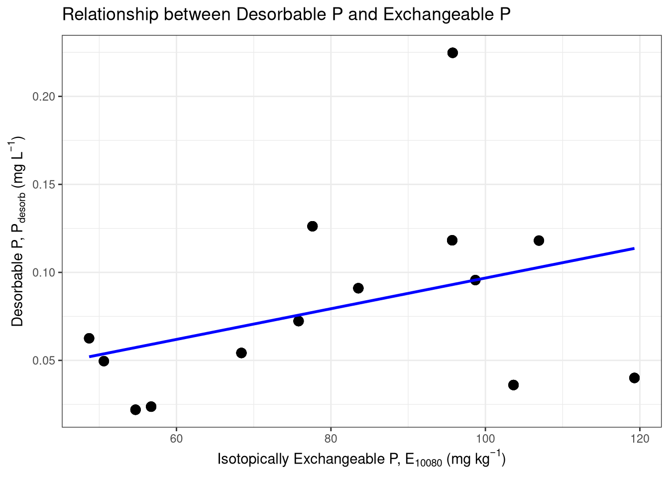
# Step 3: Perform the formal correlation test
# Using Spearman's rank correlation is a robust choice
spearman_capacity <- cor.test(correlation_data$PS, correlation_data$E_exp_10080, method = "spearman")
print("Spearman correlation between PS and E_exp_10080:")
[1] "Spearman correlation between PS and E_exp_10080:"print(spearman_capacity)
    Spearman's rank correlation rho

data:  correlation_data$PS and correlation_data$E_exp_10080
S = 145564, p-value = 5.745e-06
alternative hypothesis: true rho is not equal to 0
sample estimates:
      rho
0.4104453
# --- Kinetic Comparison (k vs. n-value) ---
# Step 2: Visualize the relationship
ggplot(correlation_data, aes(x = n_1440, y = k)) +
geom_point(size = 3, alpha = 0.7) +
geom_smooth(method = "lm", se = FALSE, color = "blue") +
labs(
title = TeX("Relationship between Desorption Rate and Exchange Rate"),
x = TeX("IEK Kinetic Parameter, $n_{60}$"),
y = TeX("Desorption Rate Constant, $k$ (min$^{-1}$)")
) +
theme_bw()`geom_smooth()` using formula = 'y ~ x'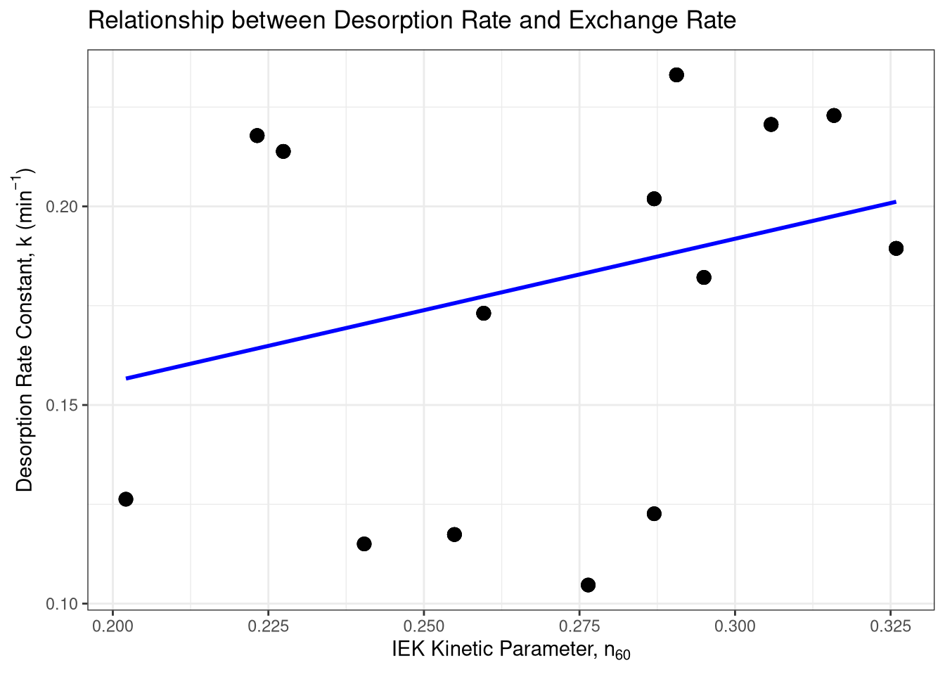
# Step 3: Perform the formal correlation test
spearman_kinetic <- cor.test(correlation_data$k, correlation_data$n_1440, method = "spearman")
print("Spearman correlation between k and n_60:")
[1] "Spearman correlation between k and n_60:"print(spearman_kinetic)
    Spearman's rank correlation rho

data:  correlation_data$k and correlation_data$n_1440
S = 155343, p-value = 4.873e-05
alternative hypothesis: true rho is not equal to 0
sample estimates:
      rho
0.3708392 D$Site |> unique()[1] Cadenazzo Ellighausen Oensingen Reckenholz Ruemlang
Levels: Cadenazzo Ellighausen Oensingen Reckenholz Ruemlangsave.image(file = "~/Documents/Master Thesis/Master-Thesis-P-kinetics/data/results_coefficient_analysis")