To explore, whether the proposed mechanisms and experiments to assess their dynamic, in a first step the Treatment levels \(0P\) and \(166P\) for all sites were analyzed. The experiments were conducted as displayed in the original paper of Flossmann & Richter with adjustments according to developments in technique and available equipment of the soil laboratory. Instead of the CAL-method, the Olsen-method was used to measure and estimate the quantity of P.
Model of P-release after Flossman & Richter
\[\frac{dP}{dt}=k\times(P^S-P)\] The constant \(P^S\) denotes the amount of semi-labile P and was originally estimated as \(P_\text{Olsen}-P_{H_2O}\). Subsequently the DE is solved exactly, since the soil is as \(t=0\) mixed with deionized water, it was assumed that \(P(0)=0\)
Exact Solution
\[P(t)=P^{\text{S}}-C\times e^{-kt}\]
for \(P(0)=P_0\) we receive:
\[P(t)=P^S-(P^S-P_0)\times e^{-kt}\]
If we set \(P(0)=0\) we receive:
\[P(t)=P^S\times(1-e^{-kt})q\]
Linearization
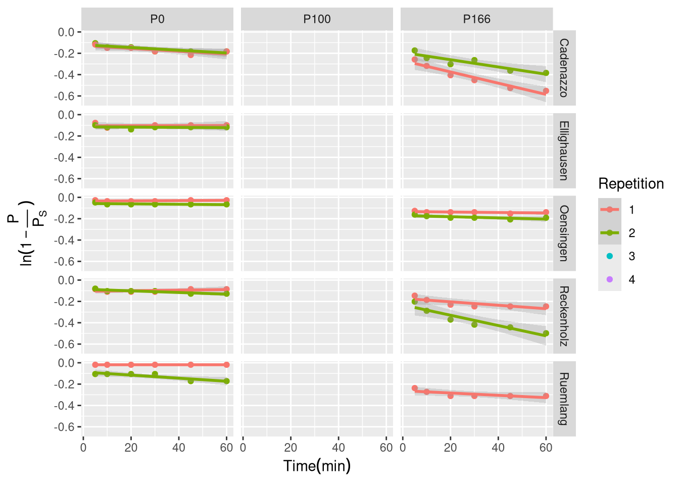
Now we linearize the DE, so that a linear model can be employed to test the relation and estimate the parameters of interest:
Now we can see, whether our linearized model displays a linear relation.
In [2]:
res <-lmList(Y1 ~ t.min. | uid, d[d$Repetition==1|d$Repetition==2,],na.action = na.pass)summary(res)
Call:
  Model: Y1 ~ t.min. | uid
   Data: d[d$Repetition == 1 | d$Repetition == 2, ]

Coefficients:
   (Intercept)
                      Estimate Std. Error    t value     Pr(>|t|)
Cadenazzo_P0_1     -0.12891945 0.01537006  -8.387702 4.332766e-12
Cadenazzo_P0_2     -0.12037045 0.01537006  -7.831491 4.433395e-11
Cadenazzo_P100_1            NA         NA         NA           NA
Cadenazzo_P100_2            NA         NA         NA           NA
Cadenazzo_P166_1   -0.26932199 0.01537006 -17.522512 6.499702e-27
Cadenazzo_P166_2   -0.19243796 0.01537006 -12.520316 2.550625e-19
Ellighausen_P0_1   -0.10464296 0.01537006  -6.808236 3.136905e-09
Ellighausen_P0_2   -0.11438112 0.01537006  -7.441815 2.257472e-10
Ellighausen_P100_1          NA         NA         NA           NA
Ellighausen_P100_2          NA         NA         NA           NA
Ellighausen_P166_1          NA         NA         NA           NA
Oensingen_P0_1     -0.03432646 0.01537006  -2.233333 2.882091e-02
Oensingen_P0_2     -0.05745952 0.01537006  -3.738407 3.819350e-04
Oensingen_P100_1            NA         NA         NA           NA
Oensingen_P100_2            NA         NA         NA           NA
Oensingen_P166_1   -0.13275856 0.01537006  -8.637481 1.527196e-12
Oensingen_P166_2   -0.17051390 0.01537006 -11.093902 6.616653e-17
Reckenholz_P0_1    -0.10545869 0.01537006  -6.861308 2.519112e-09
Reckenholz_P0_2    -0.08557888 0.01537006  -5.567897 4.753375e-07
Reckenholz_P100_1           NA         NA         NA           NA
Reckenholz_P100_2           NA         NA         NA           NA
Reckenholz_P166_1  -0.17172348 0.01537006 -11.172600 4.839473e-17
Reckenholz_P166_2  -0.23296391 0.01537006 -15.156998 1.712692e-23
Ruemlang_P0_1      -0.01851905 0.01537006  -1.204878 2.324269e-01
Ruemlang_P0_2      -0.08675331 0.01537006  -5.644307 3.515958e-07
Ruemlang_P100_1             NA         NA         NA           NA
Ruemlang_P100_2             NA         NA         NA           NA
Ruemlang_P166_1    -0.26153690 0.01537006 -17.016002 3.315417e-26
Ruemlang_P166_2             NA         NA         NA           NA
   t.min.
                        Estimate   Std. Error       t value     Pr(>|t|)
Cadenazzo_P0_1     -1.318800e-03 0.0004483906 -2.941186e+00 4.466020e-03
Cadenazzo_P0_2     -1.272378e-03 0.0004483906 -2.837654e+00 5.984783e-03
Cadenazzo_P100_1              NA           NA            NA           NA
Cadenazzo_P100_2              NA           NA            NA           NA
Cadenazzo_P166_1   -5.270369e-03 0.0004483906 -1.175397e+01 4.905164e-18
Cadenazzo_P166_2   -3.394812e-03 0.0004483906 -7.571105e+00 1.316077e-10
Ellighausen_P0_1    4.952586e-05 0.0004483906  1.104525e-01 9.123759e-01
Ellighausen_P0_2   -1.260933e-04 0.0004483906 -2.812130e-01 7.794010e-01
Ellighausen_P100_1            NA           NA            NA           NA
Ellighausen_P100_2            NA           NA            NA           NA
Ellighausen_P166_1            NA           NA            NA           NA
Oensingen_P0_1      1.049070e-04 0.0004483906  2.339634e-01 8.157164e-01
Oensingen_P0_2     -1.837559e-04 0.0004483906 -4.098121e-01 6.832320e-01
Oensingen_P100_1              NA           NA            NA           NA
Oensingen_P100_2              NA           NA            NA           NA
Oensingen_P166_1   -2.320568e-04 0.0004483906 -5.175327e-01 6.064639e-01
Oensingen_P166_2   -5.531502e-04 0.0004483906 -1.233635e+00 2.215861e-01
Reckenholz_P0_1     2.780943e-04 0.0004483906  6.202053e-01 5.371956e-01
Reckenholz_P0_2    -7.752286e-04 0.0004483906 -1.728914e+00 8.836252e-02
Reckenholz_P100_1             NA           NA            NA           NA
Reckenholz_P100_2             NA           NA            NA           NA
Reckenholz_P166_1  -1.609218e-03 0.0004483906 -3.588876e+00 6.216266e-04
Reckenholz_P166_2  -4.831330e-03 0.0004483906 -1.077482e+01 2.367928e-16
Ruemlang_P0_1       8.878899e-20 0.0004483906  1.980171e-16 1.000000e+00
Ruemlang_P0_2      -1.438957e-03 0.0004483906 -3.209160e+00 2.032261e-03
Ruemlang_P100_1               NA           NA            NA           NA
Ruemlang_P100_2               NA           NA            NA           NA
Ruemlang_P166_1    -1.090605e-03 0.0004483906 -2.432266e+00 1.764226e-02
Ruemlang_P166_2               NA           NA            NA           NA

Residual standard error: 0.02119011 on 68 degrees of freedom
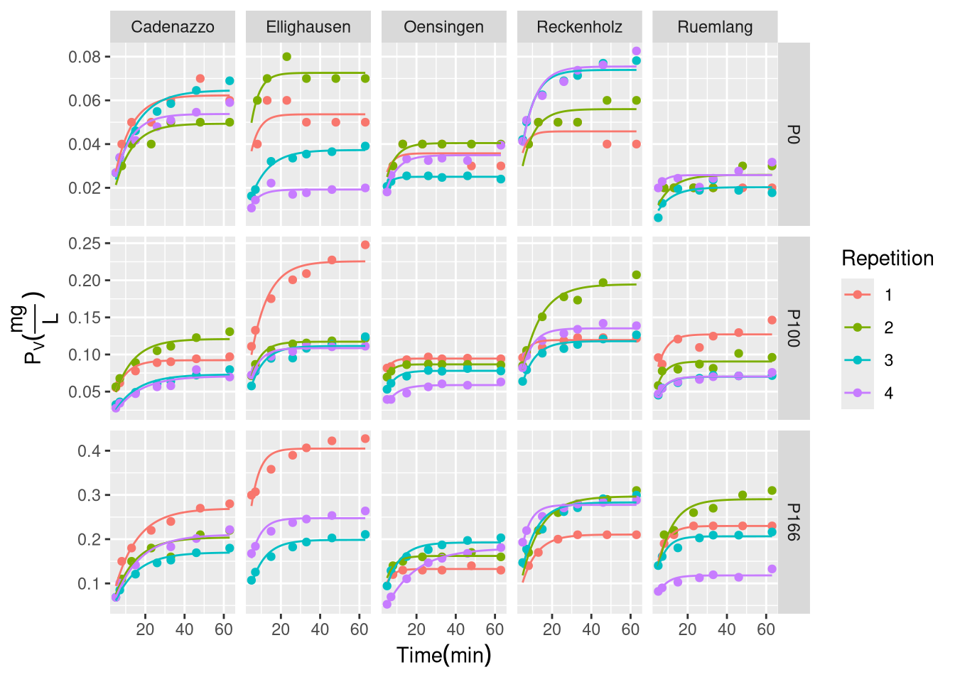
If the parameter for the plateau could be estimated directly by using a non-linear non-least-squares model, we could omit the Olsen-measurement in the future.
LG: our nls is very sensitive to moderatly high Pv.mg.L at small time points. Since the … disolves already before we start measureing, we will add 3 min to our time-measurement.
In [3]:
Res <-nlsList(Pv.mg.L. ~ PS * (1-exp(-k * (t.dt))) | uid, d[, c("Pv.mg.L.", "uid", "t.dt")], start=list(PS=0.1,k=0.2))# summary(Res)# d$nls_pred <- predict(Res)# Extract coefficients from the nlsList resultsnls_coefs <-coef(Res)nls_coefs$uid <-rownames(nls_coefs)# Merge coefficients back to the main datasetd_plot <-merge(d, nls_coefs, by ="uid")# Most straightforward approach - create curves manuallytime_seq <-seq(min(d$t.dt, na.rm =TRUE), max(d$t.dt, na.rm =TRUE), length.out =100)# Create prediction datapred_data <- d_plot %>%select(uid, Site, Treatment, Repetition, PS, k) %>%distinct() %>%crossing(t.dt = time_seq) %>%mutate(pred_Pv = PS * (1-exp(-k * (t.dt))))# Final plotp1 <-ggplot() +geom_point(data = d_plot, aes(y = Pv.mg.L., x = t.dt, col = Repetition)) +geom_line(data = pred_data, aes(x = t.dt, y = pred_Pv, col = Repetition), size =0.5) +facet_grid(Treatment ~ Site,scales ="free_y") +labs(x =TeX("$Time (min)$"),y =TeX("$P_{V}(\\frac{mg}{L})$")); suppressWarnings(print(p1))
d$ui <-interaction(d$Site, d$Treatment)nlme.coef.avg <-list()nlme.coef <-list()for (lvl inlevels(d$ui)){ d.tmp <-subset(d, ui == lvl)# first get nlsList coefs for comparison only (unused) temp_nls <-coef(nlsList(Pv.mg.L. ~ PS * (1-exp(-k * t.dt)) | uid, d.tmp[, c("Pv.mg.L.", "uid", "t.dt")], start =list(PS =0.1, k =0.2))) nlsList_coefs <-c(apply(temp_nls, 2, \(x) c(mean=mean(x), sd=sd(x))))names(nlsList_coefs) <-c("PS.mean", "PS.sd", "k.mean", "k.sd")# now do the real thing model4 <-nlme(Pv.mg.L. ~ PS * (1-exp(-k * t.dt)),fixed = PS + k ~1,random = PS + k ~1| uid,data = d.tmp[, c("Pv.mg.L.", "uid", "t.dt")],start =c(PS =0.05, k =0.12),control =nlmeControl(maxIter =200))coef(model4) fixef <- model4$coefficients$fixed ranefs <-ranef(model4)colnames(ranefs) <-paste0("ranef_",colnames(ranefs)) nlme.coef[[lvl]] <-cbind(coef(model4), ranefs, Rep=1:nrow(ranef(model4)), ui=lvl, Site=d.tmp[1, "Site"], Treatment=d.tmp[1, "Treatment"], uid =rownames(coef(model4))) nlme.coef.avg[[lvl]] <-data.frame(PS=fixef["PS"], k=fixef["k"], ui=lvl, Site=d.tmp[1, "Site"], Treatment=d.tmp[1, "Treatment"], uid = d.tmp$uid)}nlme.coef.avg <-do.call(rbind, nlme.coef.avg)# folgendes datenset wollen wir benutzen um ihn mit dem Boden zu kombinierennlme.coef <-do.call(rbind, nlme.coef)
LG: hier machen wir folgendes:
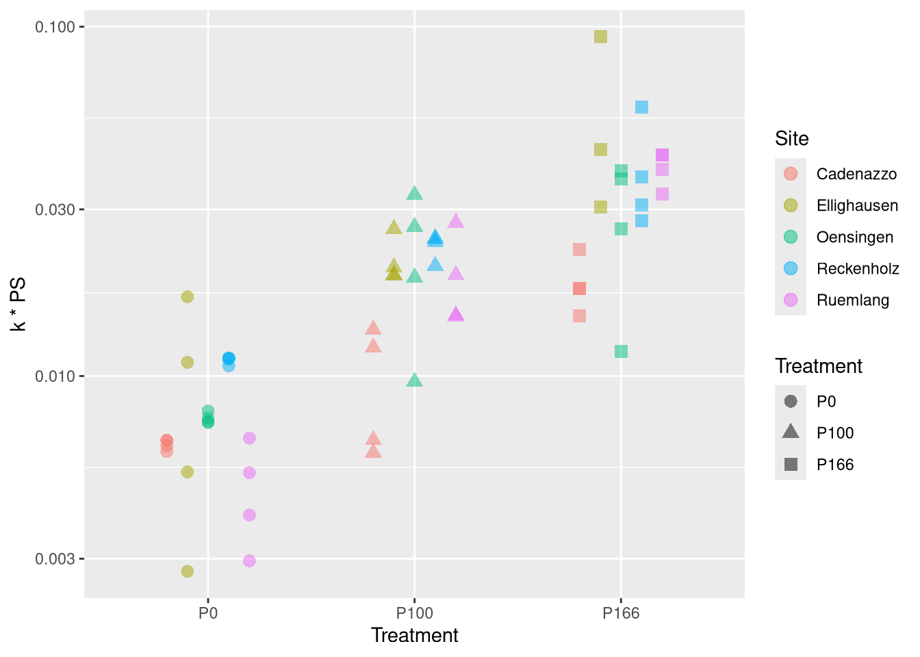
Visualisiere Daten
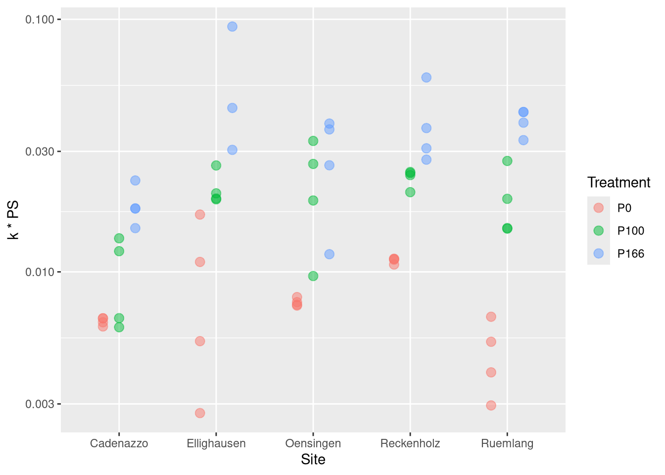
for k*PS use sqrt-scale
Erkenne, dass keine offenslichtichen verletzuungen für ein lineares modell vorhanden sind
fitte ordinary linear squares model, with Treatment as the factor of interest and Site as covariate (analougous to paired t-test and equivalent to anova with Site as block factor)
Perform a classical Type II anova (using the car::Anova function)
Perform (post-hoc) TukeyHSD test (using multcomp package)
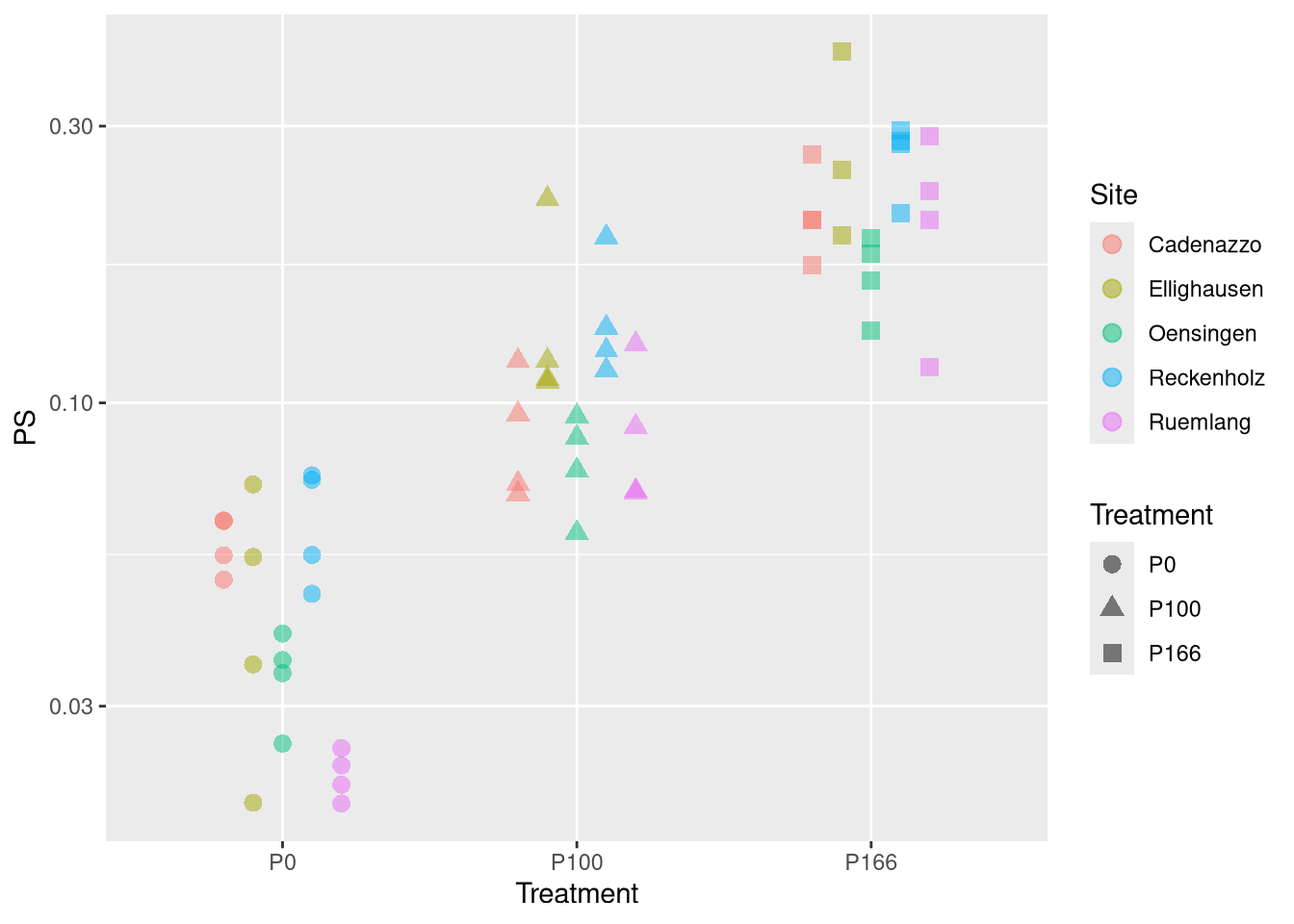
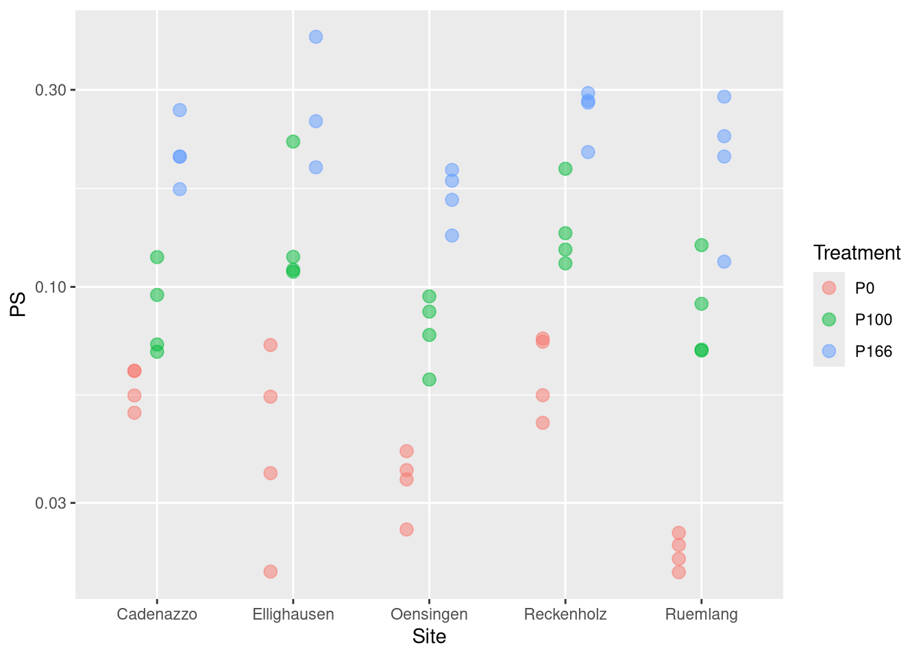
# k PS macht von der interpretation her Sinn# aber PS ist log-normal verteiltfit.PS <-lm(log(PS) ~ Treatment + Site, nlme.coef)fit.k <-lm(k ~ Treatment + Site, nlme.coef)fit.kPS <-lm(I(log(k*PS)) ~ Treatment + Site, nlme.coef)Anova(fit.PS)
Anova Table (Type II tests)

Response: log(PS)
           Sum Sq Df  F value    Pr(>F)
Treatment 27.6260  2 154.7655 < 2.2e-16 ***
Site       3.0383  4   8.5104 2.324e-05 ***
Residuals  4.6411 52
---
Signif. codes:  0 '***' 0.001 '**' 0.01 '*' 0.05 '.' 0.1 ' ' 1
summary(glht(fit.PS, mcp(Treatment ="Tukey")))
     Simultaneous Tests for General Linear Hypotheses

Multiple Comparisons of Means: Tukey Contrasts


Fit: lm(formula = log(PS) ~ Treatment + Site, data = nlme.coef)

Linear Hypotheses:
                 Estimate Std. Error t value Pr(>|t|)
P100 - P0 == 0    0.91948    0.09447   9.733   <1e-09 ***
P166 - P0 == 0    1.68127    0.09580  17.550   <1e-09 ***
P166 - P100 == 0  0.76179    0.09580   7.952   <1e-09 ***
---
Signif. codes:  0 '***' 0.001 '**' 0.01 '*' 0.05 '.' 0.1 ' ' 1
(Adjusted p values reported -- single-step method)
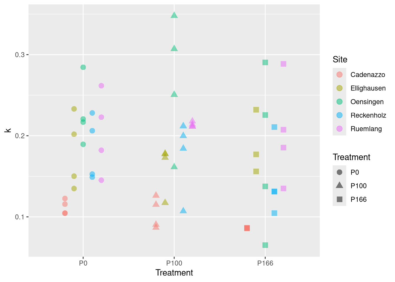
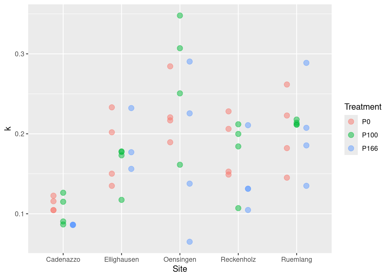
# Fazit: PS wird von treatment stark beeinfluss, k eher nicht (dafür von site)Anova(fit.k)
Anova Table (Type II tests)

Response: k
            Sum Sq Df F value    Pr(>F)
Treatment 0.007374  2  1.6124    0.2092
Site      0.108427  4 11.8547 6.442e-07 ***
Residuals 0.118902 52
---
Signif. codes:  0 '***' 0.001 '**' 0.01 '*' 0.05 '.' 0.1 ' ' 1
summary(glht(fit.k, mcp(Treatment ="Tukey")))
     Simultaneous Tests for General Linear Hypotheses

Multiple Comparisons of Means: Tukey Contrasts


Fit: lm(formula = k ~ Treatment + Site, data = nlme.coef)

Linear Hypotheses:
                  Estimate Std. Error t value Pr(>|t|)
P100 - P0 == 0    0.003111   0.015121   0.206    0.977
P166 - P0 == 0   -0.022243   0.015334  -1.451    0.323
P166 - P100 == 0 -0.025354   0.015334  -1.653    0.233
(Adjusted p values reported -- single-step method)
Anova(fit.kPS)
Anova Table (Type II tests)

Response: I(log(k * PS))
           Sum Sq Df F value    Pr(>F)
Treatment 22.4177  2 68.5970 2.609e-15 ***
Site       3.9298  4  6.0124 0.0004703 ***
Residuals  8.4969 52
---
Signif. codes:  0 '***' 0.001 '**' 0.01 '*' 0.05 '.' 0.1 ' ' 1
summary(glht(fit.kPS, mcp(Treatment ="Tukey")))
     Simultaneous Tests for General Linear Hypotheses

Multiple Comparisons of Means: Tukey Contrasts


Fit: lm(formula = I(log(k * PS)) ~ Treatment + Site, data = nlme.coef)

Linear Hypotheses:
                 Estimate Std. Error t value Pr(>|t|)
P100 - P0 == 0     0.9127     0.1278   7.140  < 1e-05 ***
P166 - P0 == 0     1.5035     0.1296  11.599  < 1e-05 ***
P166 - P100 == 0   0.5908     0.1296   4.558 8.68e-05 ***
---
Signif. codes:  0 '***' 0.001 '**' 0.01 '*' 0.05 '.' 0.1 ' ' 1
(Adjusted p values reported -- single-step method)
Results:
for PS Treatment explains a lot, and site not so much. c.f. plot for a monotonous relationship
for k, the Treatment seems to be little relevant
In [5]:
# new Data set, that gives info about SoilallP <-tryCatch(readRDS("./data/all_P.rds"))if (inherits(d, "try-error")){ allP <-tryCatch(readRDS("~/Documents/Master Thesis/Master-Thesis-P-kinetics/data/all_P.rds"))}allP$rep <- allP$rep %>%as.roman() %>%as.integer()allP$uid <-paste(allP$location,allP$treatment_ID,as.character(allP$rep),sep ="_")
In [6]:
# 1. merge this with nlme.coefsoil_data_2022 <- allP %>%filter(year ==2022) %>%select(soil_0_20_P_AAE10, soil_0_20_P_CO2,uid) %>%# Wir benennen die Spalten um, um später Konflikte zu vermeiden.rename(soil_AAE10_from_2022 = soil_0_20_P_AAE10,soil_CO2_from_2022 = soil_0_20_P_CO2 )Stycs_data <- allP %>%filter(year>=2017& year<=2022) %>%left_join(soil_data_2022, by ="uid")Stycs_data_2022 <- Stycs_data %>%mutate(soil_0_20_P_AAE10 =ifelse(year !=2022, soil_AAE10_from_2022, soil_0_20_P_AAE10),soil_0_20_P_CO2 =ifelse(year !=2022, soil_CO2_from_2022, soil_0_20_P_CO2) ) %>%# Die Hilfsspalten werden nicht mehr benötigt und können entfernt werden.select(-soil_AAE10_from_2022, -soil_CO2_from_2022)nlme.coef$kPS <- nlme.coef$k * nlme.coef$PSD <-merge(nlme.coef, Stycs_data_2022,by ="uid")D$uuid <-interaction(D$Site, D$treatment_ID, D$rep, D$year, D$crop)# rm FodderCropD <- D[D$crop !="FodderCrop",]# set wrong 0's to NAD[D$soil_0_20_P_CO2 %in%c(NA,0), "soil_0_20_P_CO2"] <-NAD[D$soil_0_20_P_AAE10 %in%c(NA,0), "soil_0_20_P_AAE10"] <-NAD[D$annual_yield_mp_DM %in%c(NA,0), "annual_yield_mp_DM"] <-NAD[D$Ymain_rel %in%c(NA,0), "Ymain_rel"] <-NAD[D$annual_P_uptake %in%c(NA,0), "annual_P_uptake"] <-NAD[D$annual_P_balance %in%c(NA,0), "annual_P_balance"] <-NA# add log-transformed versions# D$k_logPS <- D$k * log(D$PS)D$kPS_log <-log(D$kPS)D$PS_log <-log(D$PS)D$P_AAE10_log <-log(D$soil_0_20_P_AAE10)D$P_CO2_log <-log(D$soil_0_20_P_CO2)D$P_AAE10_CO2_loglog <-log(D$soil_0_20_P_AAE10) *log(D$soil_0_20_P_CO2)D$Site <-as.factor(D$Site)## Compute Ymain_norm as the median yield of P166 treatment per site, year and crop# set 0 values of annual_yield_mp_DM, Ymain_rel, annual_P_uptake, annual_P_balance to NAdd <-aggregate(annual_yield_mp_DM ~ Site+Treatment+year+crop, data=D, median, na.rm =TRUE, na.action = na.pass)# only keep P166dd <- dd[dd$Treatment =="P166",]dd$Treatment <-NULLtmp <-merge(D, dd, by =c("Site", "year", "crop"), suffixes =c("", ".norm"), sort=FALSE)nrow(tmp)
[1] 383
tmp$Ymain_norm <- tmp$annual_yield_mp_DM / tmp$annual_yield_mp_DM.norm# order tmp by uid s.t. it matches Dtmp <- tmp[match(D$uuid, tmp$uuid),]# check: cbind(tmp$uid, D$uid)D$Ymain_norm <- tmp$Ymain_normoxides <-read.csv(file ="~/Documents/Master Thesis/Master-Thesis-P-kinetics/data/oxides.csv", na.strings =c("", "n.a."))D <-left_join(D,oxides,by="ui")IEK <-read.csv(file ="~/Documents/Master Thesis/Master-Thesis-P-kinetics/data/IEK.csv", na.strings =c("", "n.a."))IEK_wide <- IEK %>%pivot_wider(id_cols = uid, # The column that uniquely identifies each samplenames_from = IEK_time, # The column containing the time points (e.g., 1, 10, 30)values_from =c(n,E_mod, rt_R, E_exp), # The columns whose values you want to spread outnames_sep ="_"# Separator for the new column names (e.g., E_exp_1, E_exp_10) )# Step 3: Inspect the new wide-format dataframe# It should now have one row per 'uid'print("First few rows of the new wide-format IEK data:")
[1] "First few rows of the new wide-format IEK data:"
head(IEK_wide)
# A tibble: 6 × 41
  uid           n_1  n_10  n_30  n_60 n_1440 n_10080 n_30240 n_1.25  n_31 n_1505
  <chr>       <dbl> <dbl> <dbl> <dbl>  <dbl>   <dbl>   <dbl>  <dbl> <dbl>  <dbl>
1 Cadenazzo…  0.266    NA    NA    NA  0.276   0.286   0.298 NA        NA     NA
2 Cadenazzo… NA        NA    NA    NA  0.287   0.295   0.318  0.272    NA     NA
3 Cadenazzo… NA        NA    NA    NA  0.202   0.220   0.244 NA        NA     NA
4 Cadenazzo…  0.237    NA    NA    NA  0.240   0.246   0.257 NA        NA     NA
5 Ruemlang_…  0.324    NA    NA    NA  0.295   0.283   0.272 NA        NA     NA
6 Ruemlang_…  0.319    NA    NA    NA  0.316   0.305   0.299 NA        NA     NA
# ℹ 30 more variables: E_mod_1 <dbl>, E_mod_10 <dbl>, E_mod_30 <dbl>,
#   E_mod_60 <dbl>, E_mod_1440 <dbl>, E_mod_10080 <dbl>, E_mod_30240 <dbl>,
#   E_mod_1.25 <dbl>, E_mod_31 <dbl>, E_mod_1505 <dbl>, rt_R_1 <dbl>,
#   rt_R_10 <dbl>, rt_R_30 <dbl>, rt_R_60 <dbl>, rt_R_1440 <dbl>,
#   rt_R_10080 <dbl>, rt_R_30240 <dbl>, rt_R_1.25 <dbl>, rt_R_31 <dbl>,
#   rt_R_1505 <dbl>, E_exp_1 <dbl>, E_exp_10 <dbl>, E_exp_30 <dbl>,
#   E_exp_60 <dbl>, E_exp_1440 <dbl>, E_exp_10080 <dbl>, E_exp_30240 <dbl>, …
print("Column names of the new wide-format IEK data:")
[1] "Column names of the new wide-format IEK data:"
# The new names will look like: "E_exp_1", "E_exp_10", "rt_R_1", "rt_R_10", etc.# Step 4: Merge the wide IEK data with your main dataframe D# Now that both have one row per uid, we can perform a clean join.D <- D %>%left_join(IEK_wide, by ="uid")#################################################### Original Comparison 1 year k,PS vs. 6 years CO2 AAE10###################################################D2 <-merge(nlme.coef, allP[allP$year>=2017,],by ="uid")D2$uuid <-interaction(D2$Site, D2$treatment_ID, D2$rep, D2$year, D2$crop)# rm FodderCropD2 <- D2[D2$crop !="FodderCrop",]# set wrong 0's to NAD2[D2$soil_0_20_P_CO2 %in%c(NA,0), "soil_0_20_P_CO2"] <-NAD2[D2$soil_0_20_P_AAE10 %in%c(NA,0), "soil_0_20_P_AAE10"] <-NAD2[D2$annual_yield_mp_DM %in%c(NA,0), "annual_yield_mp_DM"] <-NAD2[D2$Ymain_rel %in%c(NA,0), "Ymain_rel"] <-NAD2[D2$annual_P_uptake %in%c(NA,0), "annual_P_uptake"] <-NAD2[D2$annual_P_balance %in%c(NA,0), "annual_P_balance"] <-NA# add log-transformed versions# D2$k_logPS <- D2$k * log(D2$PS)D2$kPS_log <-log(D2$kPS)D2$PS_log <-log(D2$PS)D2$P_AAE10_log <-log(D2$soil_0_20_P_AAE10)D2$P_CO2_log <-log(D2$soil_0_20_P_CO2)D2$P_AAE10_CO2_loglog <-log(D2$soil_0_20_P_AAE10) *log(D2$soil_0_20_P_CO2)D2$Site <-as.factor(D2$Site)## Compute Ymain_norm as the median yield of P166 treatment per site, year and crop# set 0 values of annual_yield_mp_DM, Ymain_rel, annual_P_uptake, annual_P_balance to NAdd <-aggregate(annual_yield_mp_DM ~ Site+Treatment+year+crop, data=D2, median, na.rm =TRUE, na.action = na.pass)# only keep P166dd <- dd[dd$Treatment =="P166",]dd$Treatment <-NULLtmp <-merge(D2, dd, by =c("Site", "year", "crop"), suffixes =c("", ".norm"), sort=FALSE)nrow(tmp)
[1] 501
tmp$Ymain_norm <- tmp$annual_yield_mp_DM / tmp$annual_yield_mp_DM.norm# order tmp by uid s.t. it matches D2tmp <- tmp[match(D2$uuid, tmp$uuid),]# check: cbind(tmp$uid, D2$uid)D2$Ymain_norm <- tmp$Ymain_normoxides <-read.csv(file ="~/Documents/Master Thesis/Master-Thesis-P-kinetics/data/oxides.csv", na.strings =c("", "n.a."))D2 <-left_join(D2,oxides,by="ui")IEK <-read.csv(file ="~/Documents/Master Thesis/Master-Thesis-P-kinetics/data/IEK.csv", na.strings =c("", "n.a."))IEK_wide <- IEK %>%pivot_wider(id_cols = uid, # The column that uniquely identifies each samplenames_from = IEK_time, # The column containing the time points (e.g., 1, 10, 30)values_from =c(n,E_mod, rt_R, E_exp), # The columns whose values you want to spread outnames_sep ="_"# Separator for the new column names (e.g., E_exp_1, E_exp_10) )# Step 3: Inspect the new wide-format dataframe# It should now have one row per 'uid'print("First few rows of the new wide-format IEK data:")
[1] "First few rows of the new wide-format IEK data:"
head(IEK_wide)
# A tibble: 6 × 41
  uid           n_1  n_10  n_30  n_60 n_1440 n_10080 n_30240 n_1.25  n_31 n_1505
  <chr>       <dbl> <dbl> <dbl> <dbl>  <dbl>   <dbl>   <dbl>  <dbl> <dbl>  <dbl>
1 Cadenazzo…  0.266    NA    NA    NA  0.276   0.286   0.298 NA        NA     NA
2 Cadenazzo… NA        NA    NA    NA  0.287   0.295   0.318  0.272    NA     NA
3 Cadenazzo… NA        NA    NA    NA  0.202   0.220   0.244 NA        NA     NA
4 Cadenazzo…  0.237    NA    NA    NA  0.240   0.246   0.257 NA        NA     NA
5 Ruemlang_…  0.324    NA    NA    NA  0.295   0.283   0.272 NA        NA     NA
6 Ruemlang_…  0.319    NA    NA    NA  0.316   0.305   0.299 NA        NA     NA
# ℹ 30 more variables: E_mod_1 <dbl>, E_mod_10 <dbl>, E_mod_30 <dbl>,
#   E_mod_60 <dbl>, E_mod_1440 <dbl>, E_mod_10080 <dbl>, E_mod_30240 <dbl>,
#   E_mod_1.25 <dbl>, E_mod_31 <dbl>, E_mod_1505 <dbl>, rt_R_1 <dbl>,
#   rt_R_10 <dbl>, rt_R_30 <dbl>, rt_R_60 <dbl>, rt_R_1440 <dbl>,
#   rt_R_10080 <dbl>, rt_R_30240 <dbl>, rt_R_1.25 <dbl>, rt_R_31 <dbl>,
#   rt_R_1505 <dbl>, E_exp_1 <dbl>, E_exp_10 <dbl>, E_exp_30 <dbl>,
#   E_exp_60 <dbl>, E_exp_1440 <dbl>, E_exp_10080 <dbl>, E_exp_30240 <dbl>, …
print("Column names of the new wide-format IEK data:")
[1] "Column names of the new wide-format IEK data:"
# The new names will look like: "E_exp_1", "E_exp_10", "rt_R_1", "rt_R_10", etc.# Step 4: Merge the wide IEK data with your main dataframe D# Now that both have one row per uid, we can perform a clean join.D2 <- D2 %>%left_join(IEK_wide, by ="uid")RES$D <- DRES$D2 <- D2RES$nlme.coef.avg <- nlme.coef.avgRES$data <- dsaveRDS(RES, file ="./data/RES.rds")