The results are presented in three main parts. First, the development and validation of the phosphorus (P) desorption kinetic model are detailed, justifying the final modeling approach. Second, the descriptive trends of both agronomic outcomes and soil P parameters in response to long-term fertilization and site differences are explored visually. Finally, the predictive power of the kinetic and standard P parameters is formally evaluated using linear mixed-effects models.
Establishment of the P-Desorption Kinetic Model
The primary goal was to derive two key parameters for each soil sample: the desorbable P pool (\(P_{desorb}\)) and the rate constant (\(k\)). The analysis proceeded in two stages: an initial test of a linearized model, followed by the implementation of a more robust non-linear model.
Initial Approach: Linearized Model
Following the conceptual framework of Flossmann and Richter (1982), the first-order kinetic equation was linearized to the form \(ln(1 - P/P_{desorb}) = -kt\). For this approach, the asymptote (\(P_{desorb}\)) was not fitted but was calculated beforehand as the difference between Olsen-P and water-soluble P. A linear model was then fitted to the transformed data for each sample.
In [2]:
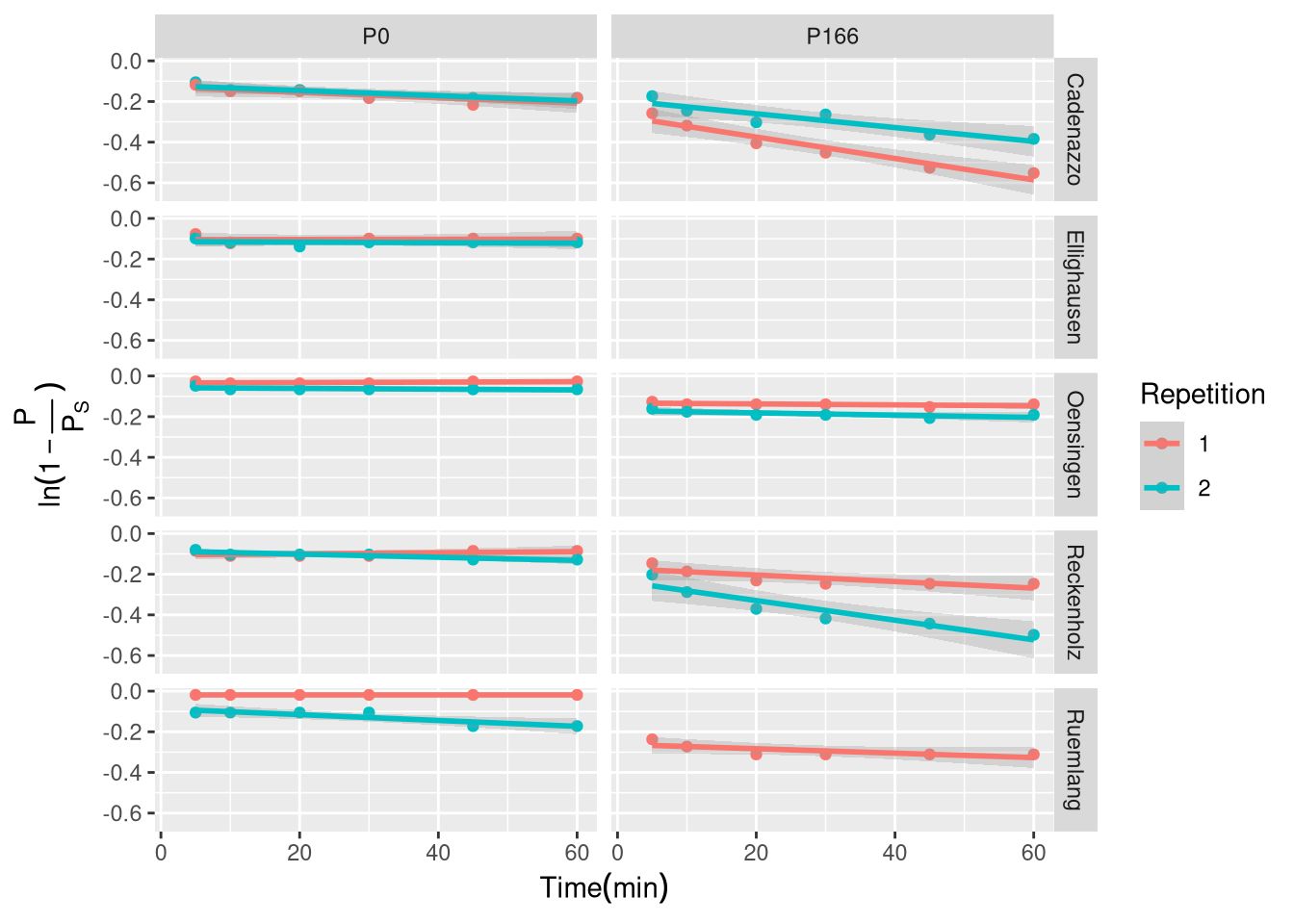
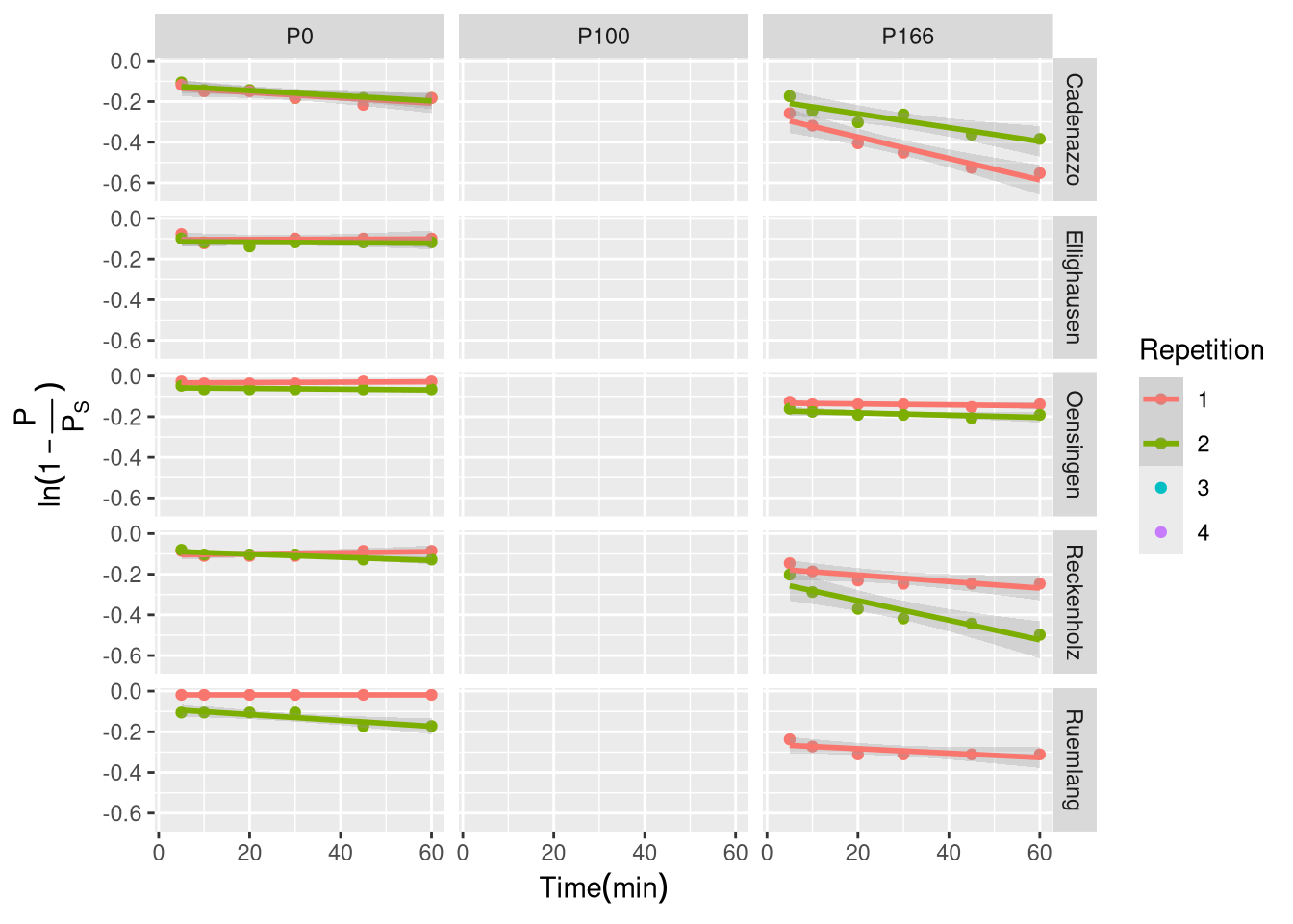
# This is a placeholder for your code from pretest.qmdggplot(d[d$Treatment!="P100"&(d$Repetition==1|d$Repetition==2),], aes(y=Y1, x=t.min., col = Repetition)) +geom_point() +facet_grid(Site ~ Treatment) +labs(x=TeX("$Time (min)$"),y=TeX("$ln(1-\\frac{P}{P_S})$")) +geom_smooth(method="lm", alpha =0.3)
`geom_smooth()` using formula = 'y ~ x'
Warning: Removed 13 rows containing non-finite outside the scale range
(`stat_smooth()`).
Warning: Removed 13 rows containing missing values or values outside the scale range
(`geom_point()`).
Test of the linearized first-order kinetic model. Data is faceted by Site and P fertilization Treatment. The solid line represents a linear model fit.
(Placeholder for the linearized model plot)
The results of this linearized approach were inconsistent (Figure X.1). While some samples showed a reasonable linear trend, many exhibited significant deviations, particularly a curvilinear pattern. Furthermore, the model required the intercept to be fixed at zero, but the statistical summary of the fitted models (lmList) showed that the estimated intercepts were often significantly different from zero (p < 0.05). For example, the sample Cadenazzo_P166_1 had a highly significant intercept of -0.27 (p < 0.001). This systematic deviation from the model’s core assumption indicated that this linearized approach, which relied on an externally estimated asymptote, was not robust for this dataset.
Final Approach: Non-Linear Model
Given the limitations of the linearized method, a direct non-linear modeling approach was adopted to estimate both \(P_{desorb}\) and \(k\) simultaneously from the untransformed data. The model \(P(t) = P_{desorb} \times (1 - e^{-k \times t'})\) was fitted to each sample’s desorption curve.
Warning: 1 error caught in nls(model, data = data, control = controlvals, start
= start): singular gradient
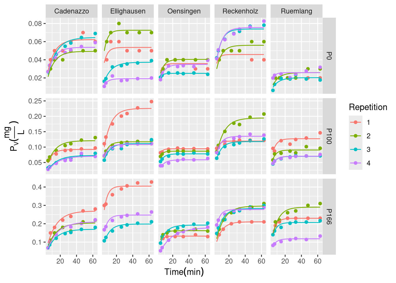
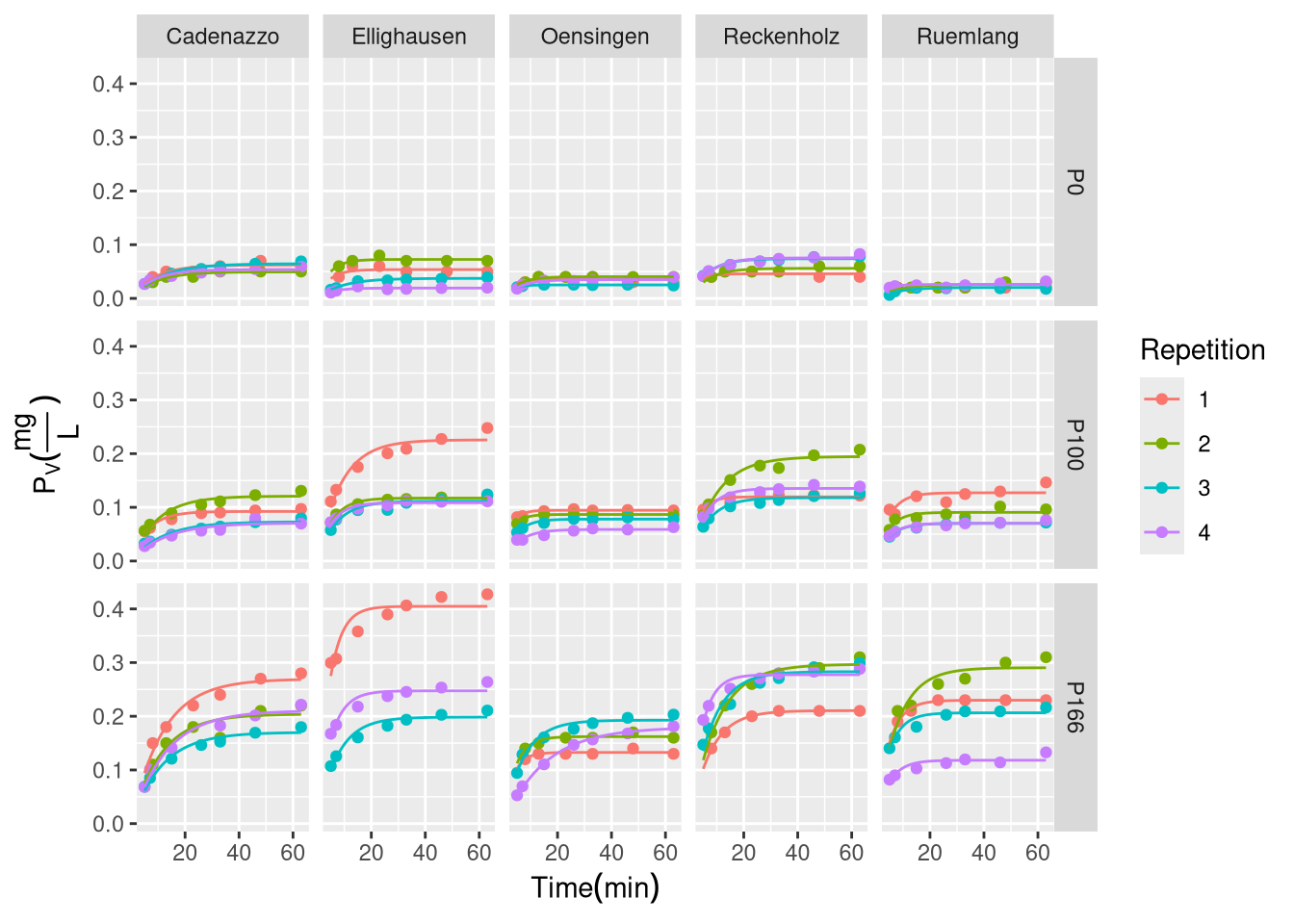
# summary(Res)# d$nls_pred <- predict(Res)# Extract coefficients from the nlsList resultsnls_coefs <-coef(Res)nls_coefs$uid <-rownames(nls_coefs)# Merge coefficients back to the main datasetd_plot <-merge(d, nls_coefs, by ="uid")# Most straightforward approach - create curves manuallytime_seq <-seq(min(d$t.dt, na.rm =TRUE), max(d$t.dt, na.rm =TRUE), length.out =100)# Create prediction datapred_data <- d_plot %>%select(uid, Site, Treatment, Repetition, PS, k) %>%distinct() %>%crossing(t.dt = time_seq) %>%mutate(pred_Pv = PS * (1-exp(-k * (t.dt))))# This is a placeholder for your code from pretest.qmd p1 <-ggplot() +geom_point(data = d_plot, aes(y = Pv.mg.L., x = t.dt, col = Repetition)) +geom_line(data = pred_data, aes(x = t.dt, y = pred_Pv, col = Repetition), size =0.5) +facet_grid(Treatment ~ Site,scales ="free_y") +labs(x =TeX("$Time (min)$"),y =TeX("$P_{V}(\\frac{mg}{L})$"));
Warning: Using `size` aesthetic for lines was deprecated in ggplot2 3.4.0.
ℹ Please use `linewidth` instead.
suppressWarnings(print(p1))
Non-linear first-order kinetic model fits for P desorption over time. Points represent measured data and solid lines represent the fitted model for each replicate.
(Placeholder for the non-linear model plot)
This approach proved to be far more successful (Figure X.2). The non-linear model was able to accurately capture the curvilinear shape of the desorption data for nearly all samples. The successful convergence of the models for each unique sample (uid) provided robust, sample-specific estimates for both the desorbable P pool (\(P_{desorb}\)) and the rate constant (\(k\)). For example, for the sample Cadenazzo_P166_1, the model estimated a \(P_{desorb}\) of 0.27 mg/L and a \(k\) of 0.086 min⁻¹, both with high statistical significance (p < 0.01).
To account for the hierarchical data structure and obtain the most reliable estimates, the final parameters were extracted from a non-linear mixed-effects model (nlme), which models the overall fixed effects for \(k\) and \(P_{desorb}\) while allowing for random variation among individual samples. These final nlme-derived coefficients were used for all subsequent analyses.
Research Questions:
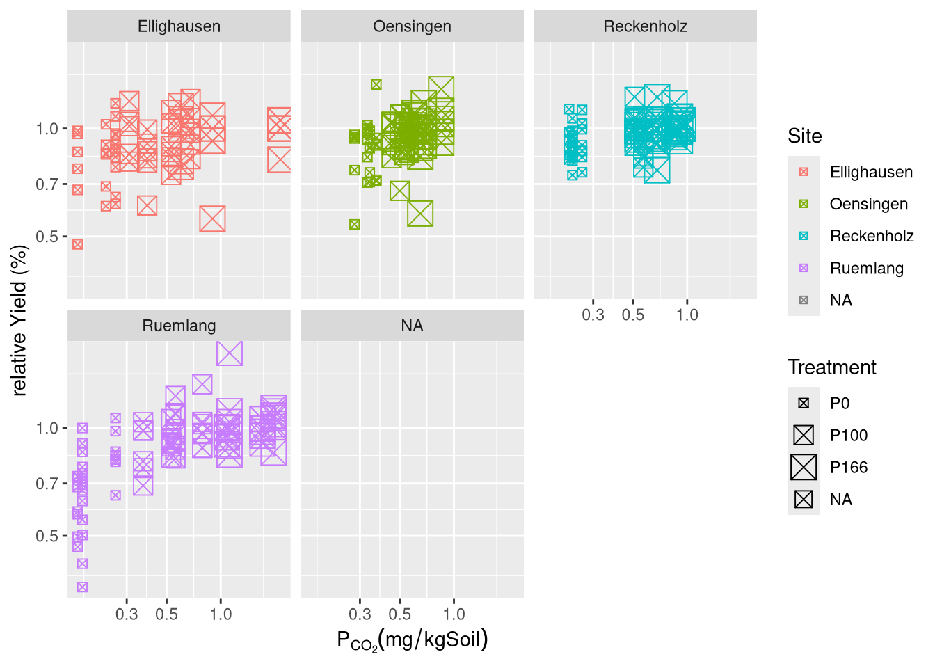
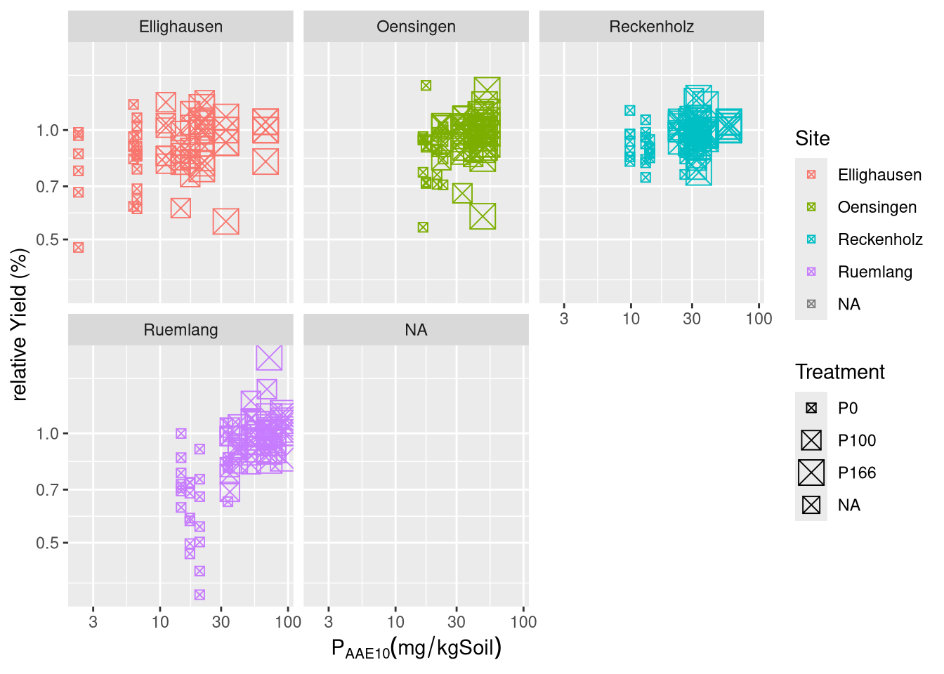
How well can current GRUD measurements of \(C_P\) predict the relative Yield, P-Uptake and P-Balance?
Hypothesis I: The measurements of the equlibrium concentrations of Phosphorus in a solvent do not display significant effects on relative Yield and consequently P-Uptake, since it is strongly dependent on yield. \(C_P\) relates strongly to the amount of Phosphorus applied, the P-balance might well be siginificantly correlated to \(C_P\) but not explain a lot of variance.
Warning: Using size for a discrete variable is not advised.
Removed 195 rows containing missing values or values outside the scale range
(`geom_point()`).
Warning: Using size for a discrete variable is not advised.
Removed 242 rows containing missing values or values outside the scale range
(`geom_point()`).
Formula contains log- or sqrt-terms.
  See help("standardize") for how such terms are standardized.
Formula contains log- or sqrt-terms.
  See help("standardize") for how such terms are standardized.
We fitted a linear mixed model (estimated using REML and nloptwrap optimizer)
to predict Ymain_rel with soil_0_20_P_CO2 and soil_0_20_P_AAE10 (formula:
Ymain_rel ~ log(soil_0_20_P_CO2) * log(soil_0_20_P_AAE10)). The model included
year as random effects (formula: list(~1 | year, ~1 | Site, ~1 | Site:block, ~1
| Site:Treatment)). The model's total explanatory power is substantial
(conditional R2 = 0.58) and the part related to the fixed effects alone
(marginal R2) is of 0.10. The model's intercept, corresponding to
soil_0_20_P_CO2 = 0 and soil_0_20_P_AAE10 = 0, is at 86.80 (95% CI [46.53,
127.06], t(203) = 4.25, p < .001). Within this model:

  - The effect of soil 0 20 P CO2 [log] is statistically non-significant and
positive (beta = 17.43, 95% CI [-6.12, 40.98], t(203) = 1.46, p = 0.146; Std.
beta = 0.84, 95% CI [-0.41, 2.09])
  - The effect of soil 0 20 P AAE10 [log] is statistically non-significant and
positive (beta = 4.59, 95% CI [-5.38, 14.56], t(203) = 0.91, p = 0.365; Std.
beta = 1.60, 95% CI [0.73, 2.48])
  - The effect of soil 0 20 P CO2 [log] × soil 0 20 P AAE10 [log] is
statistically non-significant and negative (beta = -4.37, 95% CI [-10.42,
1.67], t(203) = -1.43, p = 0.156; Std. beta = -0.93, 95% CI [-1.81, -0.04])

Standardized parameters were obtained by fitting the model on a standardized
version of the dataset. 95% Confidence Intervals (CIs) and p-values were
computed using a Wald t-distribution approximation.
report(fit.grud.Pexport)
Formula contains log- or sqrt-terms.
  See help("standardize") for how such terms are standardized.
boundary (singular) fit: see help('isSingular')
Random effect variances not available. Returned R2 does not account for random effects.
Formula contains log- or sqrt-terms.
  See help("standardize") for how such terms are standardized.
boundary (singular) fit: see help('isSingular')
Random effect variances not available. Returned R2 does not account for random effects.
We fitted a linear mixed model (estimated using REML and nloptwrap optimizer)
to predict annual_P_uptake with soil_0_20_P_CO2 and soil_0_20_P_AAE10 (formula:
annual_P_uptake ~ log(soil_0_20_P_CO2) * log(soil_0_20_P_AAE10)). The model
included year as random effects (formula: list(~1 | year, ~1 | Site, ~1 |
Site:block, ~1 | Site:Treatment)). The model's explanatory power related to the
fixed effects alone (marginal R2) is 0.18. The model's intercept, corresponding
to soil_0_20_P_CO2 = 0 and soil_0_20_P_AAE10 = 0, is at 30.63 (95% CI [8.29,
52.97], t(250) = 2.70, p = 0.007). Within this model:

  - The effect of soil 0 20 P CO2 [log] is statistically non-significant and
positive (beta = 9.82, 95% CI [-1.68, 21.32], t(250) = 1.68, p = 0.094; Std.
beta = 1.15, 95% CI [0.16, 2.15])
  - The effect of soil 0 20 P AAE10 [log] is statistically non-significant and
negative (beta = -0.81, 95% CI [-6.14, 4.52], t(250) = -0.30, p = 0.765; Std.
beta = 0.59, 95% CI [-0.06, 1.25])
  - The effect of soil 0 20 P CO2 [log] × soil 0 20 P AAE10 [log] is
statistically non-significant and negative (beta = -1.16, 95% CI [-3.95, 1.62],
t(250) = -0.82, p = 0.411; Std. beta = -0.54, 95% CI [-1.18, 0.09])

Standardized parameters were obtained by fitting the model on a standardized
version of the dataset. 95% Confidence Intervals (CIs) and p-values were
computed using a Wald t-distribution approximation.
report(fit.grud.Pbalance)
Formula contains log- or sqrt-terms.
  See help("standardize") for how such terms are standardized.
boundary (singular) fit: see help('isSingular')
Random effect variances not available. Returned R2 does not account for random effects.
Formula contains log- or sqrt-terms.
  See help("standardize") for how such terms are standardized.
boundary (singular) fit: see help('isSingular')
Random effect variances not available. Returned R2 does not account for random effects.
We fitted a linear mixed model (estimated using REML and nloptwrap optimizer)
to predict annual_P_balance with soil_0_20_P_CO2 and soil_0_20_P_AAE10
(formula: annual_P_balance ~ log(soil_0_20_P_CO2) * log(soil_0_20_P_AAE10)).
The model included year as random effects (formula: list(~1 | year, ~1 | Site,
~1 | Site:block, ~1 | Site:Treatment)). The model's explanatory power related
to the fixed effects alone (marginal R2) is 0.08. The model's intercept,
corresponding to soil_0_20_P_CO2 = 0 and soil_0_20_P_AAE10 = 0, is at -5.50
(95% CI [-36.39, 25.39], t(265) = -0.35, p = 0.726). Within this model:

  - The effect of soil 0 20 P CO2 [log] is statistically non-significant and
negative (beta = -10.40, 95% CI [-27.13, 6.33], t(265) = -1.22, p = 0.222; Std.
beta = -0.44, 95% CI [-1.26, 0.38])
  - The effect of soil 0 20 P AAE10 [log] is statistically non-significant and
positive (beta = 1.98, 95% CI [-5.24, 9.21], t(265) = 0.54, p = 0.590; Std.
beta = -0.26, 95% CI [-0.87, 0.35])
  - The effect of soil 0 20 P CO2 [log] × soil 0 20 P AAE10 [log] is
statistically non-significant and positive (beta = 1.42, 95% CI [-2.97, 5.81],
t(265) = 0.64, p = 0.526; Std. beta = 0.22, 95% CI [-0.36, 0.79])

Standardized parameters were obtained by fitting the model on a standardized
version of the dataset. 95% Confidence Intervals (CIs) and p-values were
computed using a Wald t-distribution approximation.
here I also show the non linear mixed models, following the Mitscherlich saturation curve:
In [6]:
library(nlme)# Make sure grouping variables are factorsD$year <-as.factor(D$year)D$Site <-as.factor(D$Site)D$block <-as.factor(D$block)D$crop <-as.factor(D$crop)# Fit the model# fit.mitscherlich.CO2.Yrel <- nlme(# Ymain_rel ~ A * (1 - exp(-k * soil_0_20_P_CO2 + E)), # fixed = A + k + E ~ soil_0_20_clay + soil_0_20_pH_H2O + ansum_sun + ansum_prec,# random = A ~ 1 | year/Site/block,# data = D,# subset = Treatment != "P166",# start = c(# A = 1100, A1 = 0, A2 = 0, A3 = 0, A4 = 0,# k = 0.05, k1 = 0, k2 = 0, k3 = 0, k4 = 0,# E = -3, E1 = 0, E2 = 0, E3 = 0, E4 = 0# ),# control = nlmeControl(maxIter = 500),# na.action = na.omit# )summary(fit.mitscherlich.CO2.Yrel)anova(fit.mitscherlich.CO2.Yrel)model_performance(fit.mitscherlich.CO2.Yrel)r.square.CO2 <-1-sum(residuals(fit.mitscherlich.CO2.Yrel)^2)/sum((D$Ymain_rel-mean(D$Ymain_rel,na.rm=TRUE))^2,na.rm =TRUE)# Fit the modelfit.mitscherlich.CO2.Yrel <-nlme( Ymain_rel ~ A * (1-exp(-k * kPS + E)), fixed = A + k + E ~ soil_0_20_clay + soil_0_20_pH_H2O + ansum_sun + ansum_prec,random = A ~1| year/Site/block,data = D,subset = Treatment !="P166",start =c(A =600, A1 =0, A2 =0, A3 =0, A4 =0,k =3, k1 =0, k2 =0, k3 =0, k4 =0,E =-3, E1 =0, E2 =0, E3 =0, E4 =0 ),control =nlmeControl(maxIter =1500),na.action = na.omit)summary(fit.mitscherlich.CO2.Yrel)anova(fit.mitscherlich.CO2.Yrel)model_performance(fit.mitscherlich.CO2.Yrel)r.square.CO2 <-1-sum(residuals(fit.mitscherlich.CO2.Yrel)^2)/sum((D$Ymain_rel-mean(D$Ymain_rel,na.rm=TRUE))^2,na.rm =TRUE)# fit.mitscherlich.CO2.Ynorm <- nlme(# Ymain_norm ~ A * (1 - exp(-k * kPS + E)), # fixed = A + k + E ~ soil_0_20_clay + soil_0_20_pH_H2O + ansum_sun + ansum_prec,# random = A ~ 1 | year/Site/block,# data = D,# subset = Treatment != "P166",# start = c(# A = 6, A1 = 0, A2 = 0, A3 = 0, A4 = 0,# k = 3, k1 = 0, k2 = 0, k3 = 0, k4 = 0,# E = -3, E1 = 0, E2 = 0, E3 = 0, E4 = 0# ),# control = nlmeControl(maxIter = 1500),# na.action = na.omit# )summary(fit.mitscherlich.CO2.Yrel)anova(fit.mitscherlich.CO2.Yrel)model_performance(fit.mitscherlich.CO2.Yrel)r.square.CO2 <-1-sum(residuals(fit.mitscherlich.CO2.Yrel)^2)/sum((D$Ymain_rel-mean(D$Ymain_rel,na.rm=TRUE))^2,na.rm =TRUE)# Fit the modelfit.mitscherlich.CO2.Yrel <-nlme( Ymain_norm ~ A * (1-exp(-k * soil_0_20_P_CO2 + E)), fixed = A + k + E ~ soil_0_20_clay + soil_0_20_pH_H2O + ansum_sun + ansum_prec,random = A ~1| year/Site/block,data = D,subset = Treatment !="P166",start =c(A =1100, A1 =0, A2 =0, A3 =0, A4 =0,k =0.05, k1 =0, k2 =0, k3 =0, k4 =0,E =-3, E1 =0, E2 =0, E3 =0, E4 =0 ),control =nlmeControl(maxIter =500),na.action = na.omit)summary(fit.mitscherlich.CO2.Yrel)anova(fit.mitscherlich.CO2.Yrel)model_performance(fit.mitscherlich.CO2.Yrel)r.square.CO2 <-1-sum(residuals(fit.mitscherlich.CO2.Yrel)^2)/sum((D$Ymain_rel-mean(D$Ymain_rel,na.rm=TRUE))^2,na.rm =TRUE)
With the covariate and random effect used as by Juliane Hirte we obtain , I don’t know how to interpret that, I fear that the model is overfitting data.
How do GRUD-measurements of \(C_P\) relate to the soil properties \(C_\text{org}\)-content, clay-content, silt-content and pH?
Hypothesis II: Given the known capacity of clay and silt compounds to adsorb orthophosphate a positive correlation between \(C_P\) (for both \(CO_2\) and AAE10) and silt- and clay-content. \(C_\text{org}\) has been reported to positively influence the capacity of Phosphorus as well, it is plausible it also shows a positive correlation with \(C_P\). AAE10 also deploys \(Na_4EDTA\) which is easily captured by \(Mg^{2+}\) and \(Ca^{2+}\), therefore it is officially by GRUD advised against being used in soils with \(\text{pH}>6.8\), therefore \(C_P\)-AAE10 will presumably be negatively correlated to pH.
In [7]:
anova(fit.soil.CO2)
Type III Analysis of Variance Table with Satterthwaite's method
                   Sum Sq  Mean Sq NumDF  DenDF F value Pr(>F)
soil_0_20_clay   0.017260 0.017260     1 38.410  0.1191 0.7319
soil_0_20_pH_H2O 0.080631 0.080631     1 38.254  0.5562 0.4604
soil_0_20_Corg   0.029198 0.029198     1 38.466  0.2014 0.6561
soil_0_20_silt   0.005041 0.005041     1 40.886  0.0348 0.8530
Feox             0.102556 0.102556     1 14.728  0.7074 0.4138
Alox             0.001448 0.001448     1  4.877  0.0100 0.9244
fit.soil.CO2 |>r.squaredGLMM()
           R2m       R2c
[1,] 0.1028618 0.6635412
anova(fit.soil.AAE10)
Type III Analysis of Variance Table with Satterthwaite's method
                   Sum Sq  Mean Sq NumDF  DenDF F value Pr(>F)
soil_0_20_clay   0.000000 0.000000     1 34.138  0.0000 0.9993
soil_0_20_pH_H2O 0.022655 0.022655     1 30.975  0.3822 0.5409
soil_0_20_Corg   0.091344 0.091344     1 27.873  1.5412 0.2248
soil_0_20_silt   0.033276 0.033276     1 34.322  0.5614 0.4588
Feox             0.023984 0.023984     1  7.835  0.4047 0.5428
Alox             0.104053 0.104053     1  3.886  1.7556 0.2577
fit.soil.AAE10 |>r.squaredGLMM()
           R2m       R2c
[1,] 0.2849305 0.8808985
Can the Inclusion of the net-release-kinetic of Orthophosphate improve the model power of predicting relative Yield, P-Uptake and P-Balance?
Hypothesis III: Given the comparably low solubility of \(PO_4^{3-}\) in the water-soil interface, most P is transported to the rhizosphere via diffusion. As a consequence the intensity of \(PO_4^{3-}\) might not adequately account for the P-uptake in the harvested plant. Since the diffusion process is in its velocity a kinetic and in its finally reached intensity a thermodynamic process, the inclusion of kinetic parameters might well improve the performance.
With the covariate and random effect used as by Juliane Hirte we obtain I don’t know how to interpret that, I fear that the model is overfitting data, the same might be true for the model that used \(k\times PS\) as a predictor with .
I also tried more conservative models, where I log-transformed the concentrations and PS, also I was more cautious with random effects. This resulted in coefficients that were not as straight-forward as the mitscherlich coefficients to interpret.
In [9]:
# relative Yieldanova(fit.kin.Yrel)
Type III Analysis of Variance Table with Satterthwaite's method
          Sum Sq Mean Sq NumDF  DenDF F value  Pr(>F)
k         7760.6  7760.6     1 301.92  5.7850 0.01676 *
log(PS)   5373.3  5373.3     1 302.30  4.0054 0.04625 *
k:log(PS) 8701.9  8701.9     1 302.51  6.4866 0.01136 *
---
Signif. codes:  0 '***' 0.001 '**' 0.01 '*' 0.05 '.' 0.1 ' ' 1
summary(fit.kin.Yrel)
Linear mixed model fit by REML. t-tests use Satterthwaite's method [
lmerModLmerTest]
Formula: Ymain_rel ~ k * log(PS) + (1 | year) + (1 | Site) + (1 | Site:block)
   Data: D

REML criterion at convergence: 3142.9

Scaled residuals:
    Min      1Q  Median      3Q     Max
-3.7440 -0.3919 -0.0424  0.3568  4.0380

Random effects:
 Groups     Name        Variance Std.Dev.
 Site:block (Intercept)    0.0    0.00
 year       (Intercept) 1131.6   33.64
 Site       (Intercept)  234.2   15.30
 Residual               1341.5   36.63
Number of obs: 313, groups:  Site:block, 20; year, 7; Site, 5

Fixed effects:
            Estimate Std. Error      df t value Pr(>|t|)
(Intercept)   82.385     25.976  73.506   3.172  0.00221 **
k            294.257    122.342 301.916   2.405  0.01676 *
log(PS)      -18.957      9.472 302.300  -2.001  0.04625 *
k:log(PS)    131.381     51.585 302.513   2.547  0.01136 *
---
Signif. codes:  0 '***' 0.001 '**' 0.01 '*' 0.05 '.' 0.1 ' ' 1

Correlation of Fixed Effects:
          (Intr) k      lg(PS)
k         -0.787
log(PS)    0.773 -0.870
k:log(PS) -0.748  0.933 -0.955
optimizer (nloptwrap) convergence code: 0 (OK)
boundary (singular) fit: see help('isSingular')
fit.kin.Yrel |>r.squaredGLMM()
            R2m       R2c
[1,] 0.01503741 0.5119295
# P-Uptakeanova(fit.kin.Pexport)
Type III Analysis of Variance Table with Satterthwaite's method
          Sum Sq Mean Sq NumDF  DenDF F value Pr(>F)
k         45.672  45.672     1 294.59  0.5847 0.4451
log(PS)   84.870  84.870     1 295.00  1.0866 0.2981
k:log(PS) 50.311  50.311     1 295.03  0.6441 0.4229
summary(fit.kin.Pexport)
Linear mixed model fit by REML. t-tests use Satterthwaite's method [
lmerModLmerTest]
Formula: annual_P_uptake ~ k * log(PS) + (1 | year) + (1 | Site) + (1 |
    Site:block)
   Data: D

REML criterion at convergence: 2246.3

Scaled residuals:
    Min      1Q  Median      3Q     Max
-3.2117 -0.4503 -0.0157  0.3557  4.7009

Random effects:
 Groups     Name        Variance Std.Dev.
 Site:block (Intercept)   0.00    0.000
 year       (Intercept) 114.37   10.695
 Site       (Intercept) 142.00   11.916
 Residual                78.11    8.838
Number of obs: 309, groups:  Site:block, 19; year, 7; Site, 5

Fixed effects:
            Estimate Std. Error      df t value Pr(>|t|)
(Intercept)   38.072      8.813  19.155   4.320 0.000363 ***
k             23.502     30.734 294.594   0.765 0.445074
log(PS)        2.608      2.502 295.003   1.042 0.298082
k:log(PS)     10.549     13.144 295.027   0.803 0.422866
---
Signif. codes:  0 '***' 0.001 '**' 0.01 '*' 0.05 '.' 0.1 ' ' 1

Correlation of Fixed Effects:
          (Intr) k      lg(PS)
k         -0.615
log(PS)    0.607 -0.897
k:log(PS) -0.591  0.944 -0.965
optimizer (nloptwrap) convergence code: 0 (OK)
boundary (singular) fit: see help('isSingular')
fit.kin.Pexport |>r.squaredGLMM()
            R2m       R2c
[1,] 0.04012948 0.7758557
anova(fit.kin.Pbalance)
Type III Analysis of Variance Table with Satterthwaite's method
          Sum Sq Mean Sq NumDF  DenDF F value    Pr(>F)
k          124.7   124.7     1 275.62  0.6004    0.4391
log(PS)   4906.5  4906.5     1 285.15 23.6264 1.935e-06 ***
k:log(PS)  120.8   120.8     1 280.10  0.5819    0.4462
---
Signif. codes:  0 '***' 0.001 '**' 0.01 '*' 0.05 '.' 0.1 ' ' 1
summary(fit.kin.Pbalance)
Linear mixed model fit by REML. t-tests use Satterthwaite's method [
lmerModLmerTest]
Formula: annual_P_balance ~ k * log(PS) + (1 | year) + (1 | Site) + (1 |
    Site:block)
   Data: D

REML criterion at convergence: 2719.8

Scaled residuals:
    Min      1Q  Median      3Q     Max
-4.3960 -0.5775  0.0036  0.5915  2.8874

Random effects:
 Groups     Name        Variance Std.Dev.
 Site:block (Intercept)  27.20    5.216
 year       (Intercept)  54.22    7.363
 Site       (Intercept) 127.50   11.292
 Residual               207.67   14.411
Number of obs: 330, groups:  Site:block, 20; year, 7; Site, 5

Fixed effects:
            Estimate Std. Error      df t value Pr(>|t|)
(Intercept)   59.223     11.538  62.390   5.133 3.02e-06 ***
k             42.436     54.765 275.615   0.775    0.439
log(PS)       21.577      4.439 285.149   4.861 1.93e-06 ***
k:log(PS)     17.933     23.508 280.101   0.763    0.446
---
Signif. codes:  0 '***' 0.001 '**' 0.01 '*' 0.05 '.' 0.1 ' ' 1

Correlation of Fixed Effects:
          (Intr) k      lg(PS)
k         -0.827
log(PS)    0.807 -0.897
k:log(PS) -0.792  0.941 -0.970
fit.kin.Pbalance |>r.squaredGLMM()
           R2m       R2c
[1,] 0.4896394 0.7455866
Are the kinetic coefficients \(k\) and \(PS\)(\(k\) can be interpreted as the relative speed of desorption, \(PS\) is the equilibrium concentration of \(PO_4^{3-}\) of the observed desorption in the dried fine earth-water suspension 1:20 by weight) related to soil properties?
Hypothesis IV: Clay particles as well as organic compounds with negative surface charges provide surfaces for P-sorption, especially their structure, but in general their respective concentration in a soil can be expected to significantly influence the kinetic and thermodynamic of the P-desorption reaction. The \(pH\) dictates the form of orthophosphate, with \(pH<6.5\), the predominant form will be \(H_2PO_4^-\), this should reduce electrical interactions and increase the movement- and therefore diffusion-speed.
In [10]:
anova(fit.soil.PS)
Type III Analysis of Variance Table with Satterthwaite's method
                   Sum Sq  Mean Sq NumDF  DenDF F value  Pr(>F)
soil_0_20_clay   0.002083 0.002083     1 38.033  0.0569 0.81272
soil_0_20_pH_H2O 0.000134 0.000134     1 37.384  0.0037 0.95203
soil_0_20_Corg   0.161222 0.161222     1 31.905  4.4045 0.04385 *
soil_0_20_silt   0.004846 0.004846     1 38.673  0.1324 0.71793
Feox             0.001149 0.001149     1  0.347  0.0314 0.91632
Alox             0.012358 0.012358     1  0.257  0.3376 0.79220
---
Signif. codes:  0 '***' 0.001 '**' 0.01 '*' 0.05 '.' 0.1 ' ' 1
summary(glht(fit.soil.PS))
Warning in RET$pfunction("adjusted", ...): Completion with error > abseps
Warning in RET$pfunction("adjusted", ...): Completion with error > abseps
Type III Analysis of Variance Table with Satterthwaite's method
                  Sum Sq Mean Sq NumDF  DenDF F value   Pr(>F)
soil_0_20_clay   0.27383 0.27383     1 37.930  3.2642 0.078745 .
soil_0_20_pH_H2O 0.00989 0.00989     1 37.703  0.1179 0.733211
soil_0_20_Corg   0.63137 0.63137     1 32.625  7.5263 0.009799 **
soil_0_20_silt   0.00591 0.00591     1 39.206  0.0705 0.791988
Feox             0.04311 0.04311     1  0.225  0.5139 0.775407
Alox             0.00881 0.00881     1  0.130  0.1050 0.904677
---
Signif. codes:  0 '***' 0.001 '**' 0.01 '*' 0.05 '.' 0.1 ' ' 1
summary(glht(fit.soil.kPS))
Warning in RET$pfunction("adjusted", ...): Completion with error > abseps
Warning in RET$pfunction("adjusted", ...): Completion with error > abseps
Warning in RET$pfunction("adjusted", ...): Completion with error > abseps
Is the method presented by Flossmann and Richter (1982) with the double extraction replicable with the soils from the STYCS-trial?
Hypothesis V: The authors expect the desorption kinetics to follow a 1. order kinetic, with the relation: \[ \frac{dP}{dt}=PS(1-e^{-kt})\] where \(PS\) is estimated as \(PS=[P_\text{Olsen/CAL}]-[P_{H_2O}]\), denoted as the semi-labile P-pool. The Olsen- and CAL-method deploy extractants that increase the solubility by more than order of magnitude. This presents the problem, that the estimation of \(PS\) is likely to high. It was chosen by the authors in order to make the equation linearizable, so if the linearization is not well behaved, a non-linear regression might deliver a better estimation of both parameters.
In [11]:
res <-lmList(Y1 ~ t.min. | uid, d[d$Repetition==1|d$Repetition==2,],na.action = na.pass)
Warning: 12 times caught the same error in lm.fit(x, y, offset = offset,
singular.ok = singular.ok, ...): NA/NaN/Inf in 'y'
summary(res)
Warning in summary.lm(el): essentially perfect fit: summary may be unreliable
Call:
  Model: Y1 ~ t.min. | uid
   Data: d[d$Repetition == 1 | d$Repetition == 2, ]

Coefficients:
   (Intercept)
                      Estimate Std. Error    t value     Pr(>|t|)
Cadenazzo_P0_1     -0.12891945 0.01537006  -8.387702 4.332766e-12
Cadenazzo_P0_2     -0.12037045 0.01537006  -7.831491 4.433395e-11
Cadenazzo_P100_1            NA         NA         NA           NA
Cadenazzo_P100_2            NA         NA         NA           NA
Cadenazzo_P166_1   -0.26932199 0.01537006 -17.522512 6.499702e-27
Cadenazzo_P166_2   -0.19243796 0.01537006 -12.520316 2.550625e-19
Ellighausen_P0_1   -0.10464296 0.01537006  -6.808236 3.136905e-09
Ellighausen_P0_2   -0.11438112 0.01537006  -7.441815 2.257472e-10
Ellighausen_P100_1          NA         NA         NA           NA
Ellighausen_P100_2          NA         NA         NA           NA
Ellighausen_P166_1          NA         NA         NA           NA
Oensingen_P0_1     -0.03432646 0.01537006  -2.233333 2.882091e-02
Oensingen_P0_2     -0.05745952 0.01537006  -3.738407 3.819350e-04
Oensingen_P100_1            NA         NA         NA           NA
Oensingen_P100_2            NA         NA         NA           NA
Oensingen_P166_1   -0.13275856 0.01537006  -8.637481 1.527196e-12
Oensingen_P166_2   -0.17051390 0.01537006 -11.093902 6.616653e-17
Reckenholz_P0_1    -0.10545869 0.01537006  -6.861308 2.519112e-09
Reckenholz_P0_2    -0.08557888 0.01537006  -5.567897 4.753375e-07
Reckenholz_P100_1           NA         NA         NA           NA
Reckenholz_P100_2           NA         NA         NA           NA
Reckenholz_P166_1  -0.17172348 0.01537006 -11.172600 4.839473e-17
Reckenholz_P166_2  -0.23296391 0.01537006 -15.156998 1.712692e-23
Ruemlang_P0_1      -0.01851905 0.01537006  -1.204878 2.324269e-01
Ruemlang_P0_2      -0.08675331 0.01537006  -5.644307 3.515958e-07
Ruemlang_P100_1             NA         NA         NA           NA
Ruemlang_P100_2             NA         NA         NA           NA
Ruemlang_P166_1    -0.26153690 0.01537006 -17.016002 3.315417e-26
Ruemlang_P166_2             NA         NA         NA           NA
   t.min.
                        Estimate   Std. Error       t value     Pr(>|t|)
Cadenazzo_P0_1     -1.318800e-03 0.0004483906 -2.941186e+00 4.466020e-03
Cadenazzo_P0_2     -1.272378e-03 0.0004483906 -2.837654e+00 5.984783e-03
Cadenazzo_P100_1              NA           NA            NA           NA
Cadenazzo_P100_2              NA           NA            NA           NA
Cadenazzo_P166_1   -5.270369e-03 0.0004483906 -1.175397e+01 4.905164e-18
Cadenazzo_P166_2   -3.394812e-03 0.0004483906 -7.571105e+00 1.316077e-10
Ellighausen_P0_1    4.952586e-05 0.0004483906  1.104525e-01 9.123759e-01
Ellighausen_P0_2   -1.260933e-04 0.0004483906 -2.812130e-01 7.794010e-01
Ellighausen_P100_1            NA           NA            NA           NA
Ellighausen_P100_2            NA           NA            NA           NA
Ellighausen_P166_1            NA           NA            NA           NA
Oensingen_P0_1      1.049070e-04 0.0004483906  2.339634e-01 8.157164e-01
Oensingen_P0_2     -1.837559e-04 0.0004483906 -4.098121e-01 6.832320e-01
Oensingen_P100_1              NA           NA            NA           NA
Oensingen_P100_2              NA           NA            NA           NA
Oensingen_P166_1   -2.320568e-04 0.0004483906 -5.175327e-01 6.064639e-01
Oensingen_P166_2   -5.531502e-04 0.0004483906 -1.233635e+00 2.215861e-01
Reckenholz_P0_1     2.780943e-04 0.0004483906  6.202053e-01 5.371956e-01
Reckenholz_P0_2    -7.752286e-04 0.0004483906 -1.728914e+00 8.836252e-02
Reckenholz_P100_1             NA           NA            NA           NA
Reckenholz_P100_2             NA           NA            NA           NA
Reckenholz_P166_1  -1.609218e-03 0.0004483906 -3.588876e+00 6.216266e-04
Reckenholz_P166_2  -4.831330e-03 0.0004483906 -1.077482e+01 2.367928e-16
Ruemlang_P0_1       8.878899e-20 0.0004483906  1.980171e-16 1.000000e+00
Ruemlang_P0_2      -1.438957e-03 0.0004483906 -3.209160e+00 2.032261e-03
Ruemlang_P100_1               NA           NA            NA           NA
Ruemlang_P100_2               NA           NA            NA           NA
Ruemlang_P166_1    -1.090605e-03 0.0004483906 -2.432266e+00 1.764226e-02
Ruemlang_P166_2               NA           NA            NA           NA

Residual standard error: 0.02119011 on 68 degrees of freedom
Warning: 1 error caught in nls(model, data = data, control = controlvals, start
= start): singular gradient
# summary(Res)# d$nls_pred <- predict(Res)# Extract coefficients from the nlsList resultsnls_coefs <-coef(Res)nls_coefs$uid <-rownames(nls_coefs)# Merge coefficients back to the main datasetd_plot <-merge(d, nls_coefs, by ="uid")# Most straightforward approach - create curves manuallytime_seq <-seq(min(d$t.dt, na.rm =TRUE), max(d$t.dt, na.rm =TRUE), length.out =100)# Create prediction datapred_data <- d_plot %>%select(uid, Site, Treatment, Repetition, PS, k) %>%distinct() %>%crossing(t.dt = time_seq) %>%mutate(pred_Pv = PS * (1-exp(-k * (t.dt))))# Final plotp1 <-ggplot() +geom_point(data = d_plot, aes(y = Pv.mg.L., x = t.dt, col = Repetition)) +geom_line(data = pred_data, aes(x = t.dt, y = pred_Pv, col = Repetition), size =0.5) +facet_grid(Treatment ~ Site) +labs(x =TeX("$Time (min)$"),y =TeX("$P_{V}(\\frac{mg}{L})$")); suppressWarnings(print(p1))
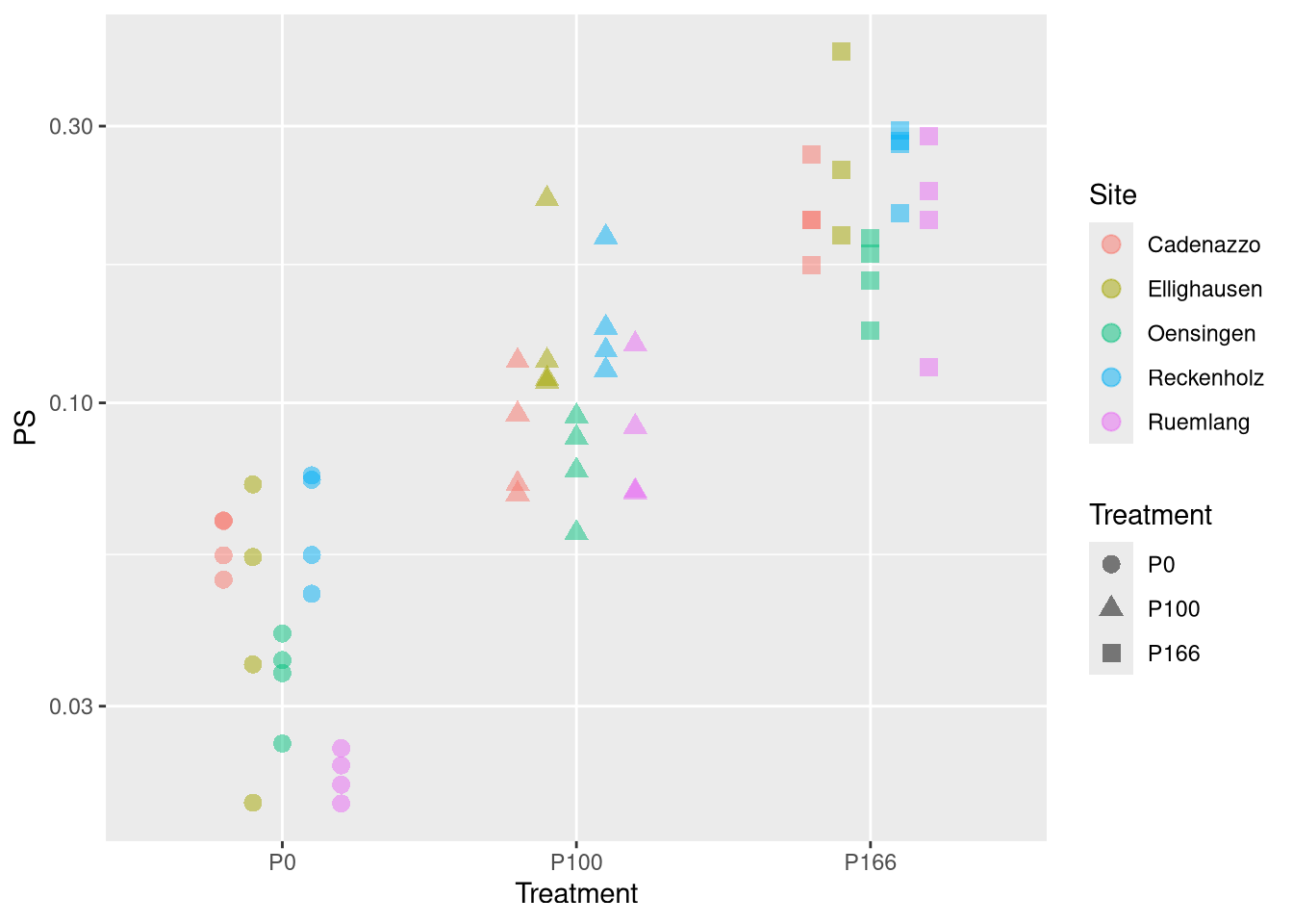
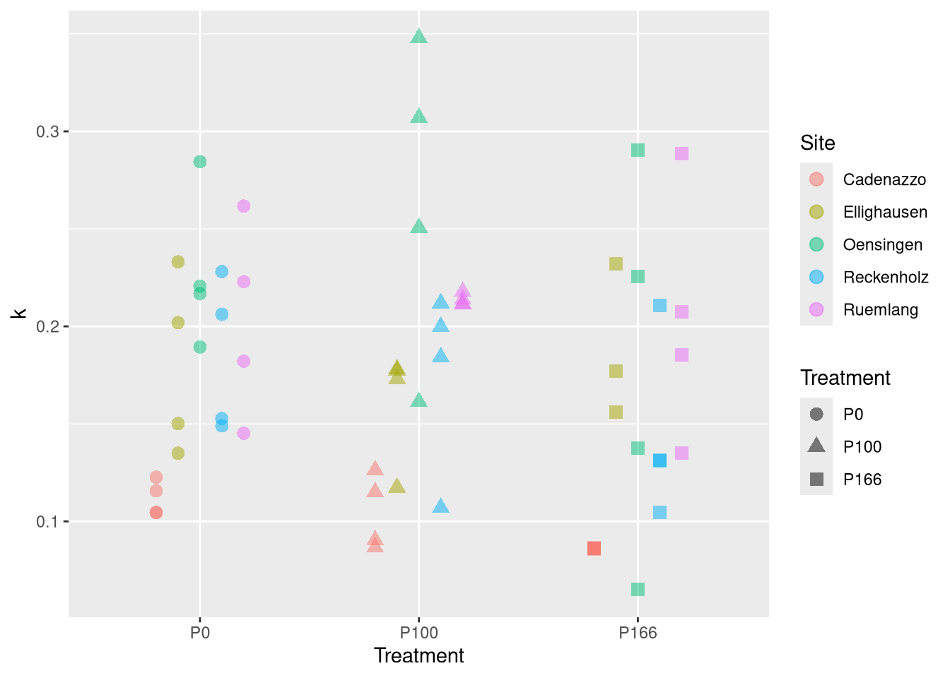
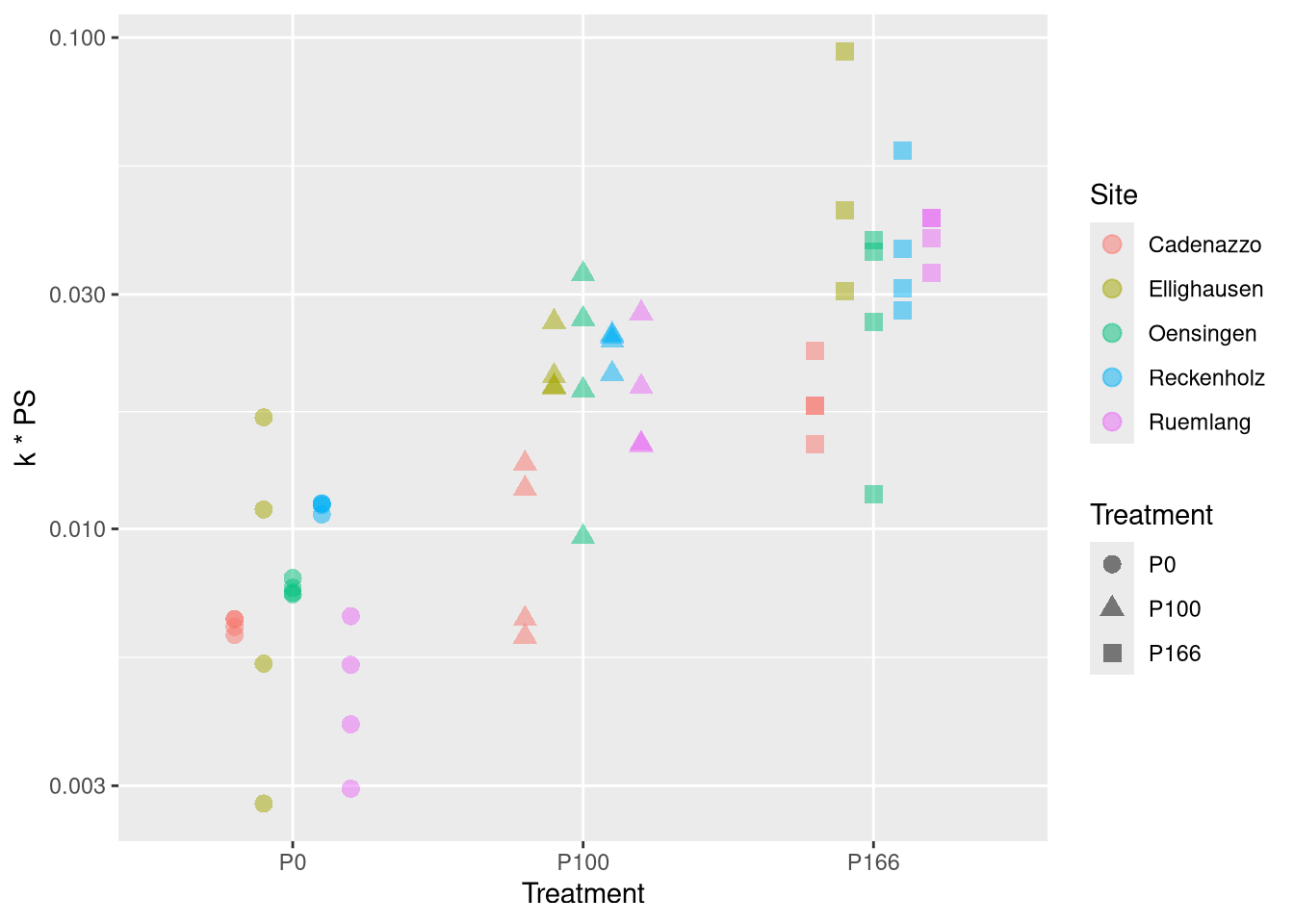
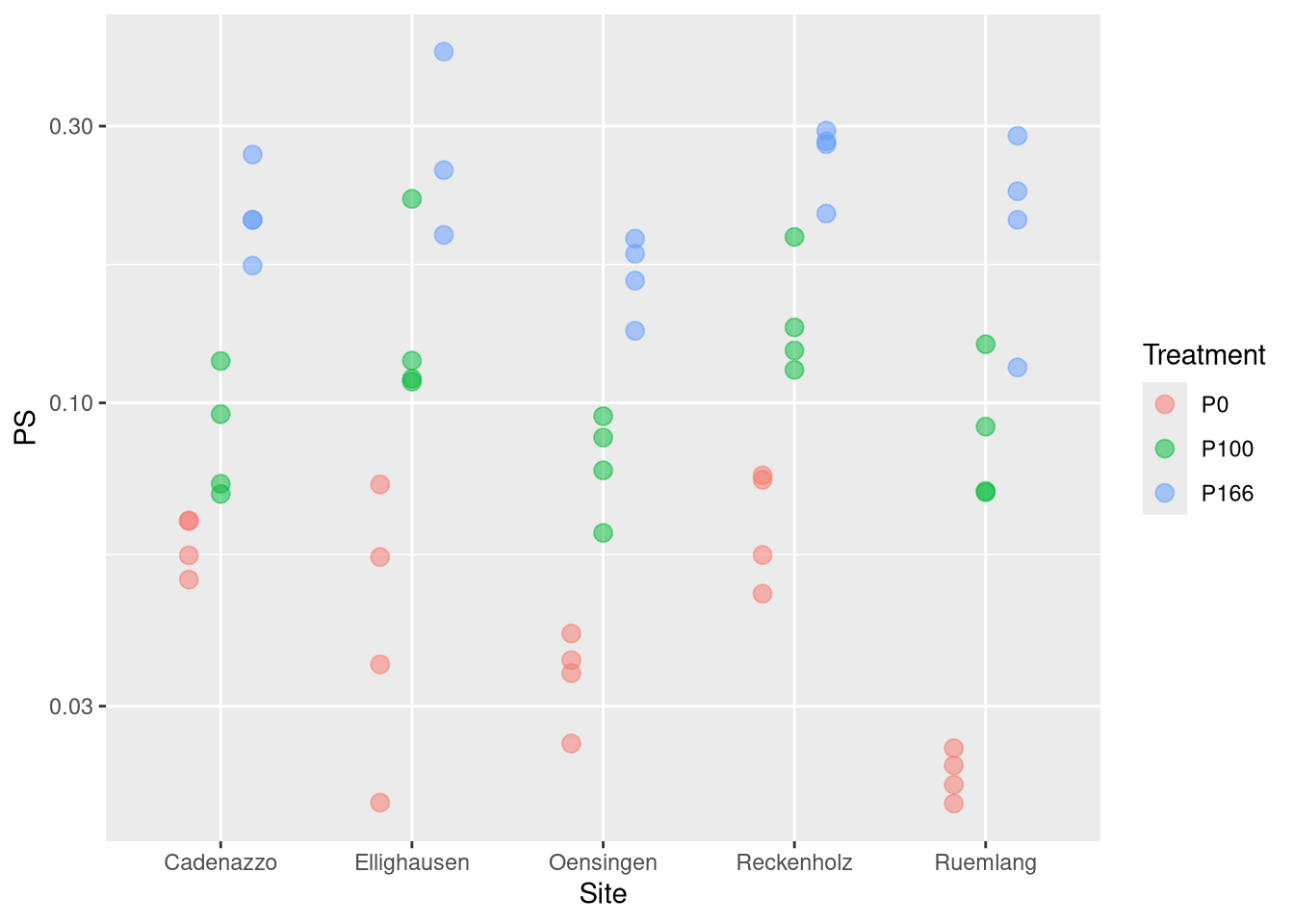
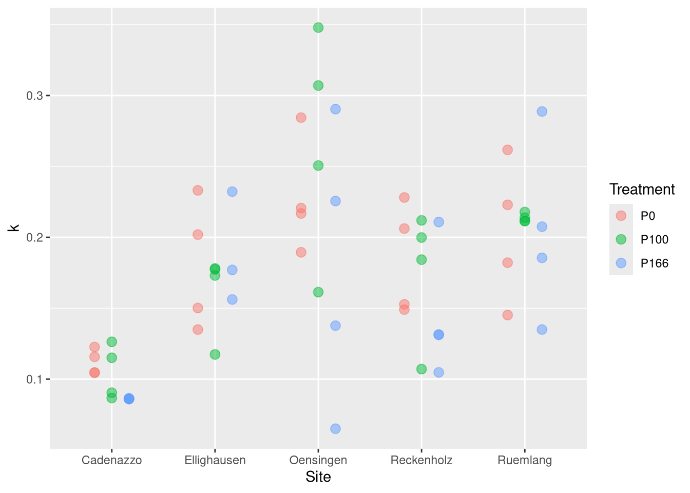
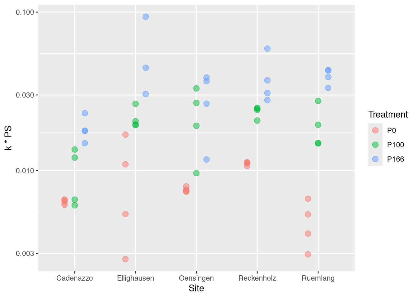
Now we see how those parameters depend on the tratment:
In [13]:
d$ui <-interaction(d$Site, d$Treatment)nlme.coef.avg <-list()nlme.coef <-list()for (lvl inlevels(d$ui)){ d.tmp <-subset(d, ui == lvl)# first get nlsList coefs for comparison only (unused) temp_nls <-coef(nlsList(Pv.mg.L. ~ PS * (1-exp(-k * t.dt)) | uid, d.tmp[, c("Pv.mg.L.", "uid", "t.dt")], start =list(PS =0.1, k =0.2))) nlsList_coefs <-c(apply(temp_nls, 2, \(x) c(mean=mean(x), sd=sd(x))))names(nlsList_coefs) <-c("PS.mean", "PS.sd", "k.mean", "k.sd")# now do the real thing model4 <-nlme(Pv.mg.L. ~ PS * (1-exp(-k * t.dt)),fixed = PS + k ~1,random = PS + k ~1| uid,data = d.tmp[, c("Pv.mg.L.", "uid", "t.dt")],start =c(PS =0.05, k =0.12),control =nlmeControl(maxIter =200))coef(model4) fixef <- model4$coefficients$fixed ranefs <-ranef(model4)colnames(ranefs) <-paste0("ranef_",colnames(ranefs)) nlme.coef[[lvl]] <-cbind(coef(model4), ranefs, Rep=1:nrow(ranef(model4)), ui=lvl, Site=d.tmp[1, "Site"], Treatment=d.tmp[1, "Treatment"], uid =rownames(coef(model4))) nlme.coef.avg[[lvl]] <-data.frame(PS=fixef["PS"], k=fixef["k"], ui=lvl, Site=d.tmp[1, "Site"], Treatment=d.tmp[1, "Treatment"], uid = d.tmp$uid)}
Warning in nlme.formula(Pv.mg.L. ~ PS * (1 - exp(-k * t.dt)), fixed = PS + :
Iteration 1, LME step: nlminb() did not converge (code = 1). Do increase
'msMaxIter'!
Warning in data.frame(PS = fixef["PS"], k = fixef["k"], ui = lvl, Site =
d.tmp[1, : row names were found from a short variable and have been discarded
Warning in data.frame(PS = fixef["PS"], k = fixef["k"], ui = lvl, Site =
d.tmp[1, : row names were found from a short variable and have been discarded
Warning in data.frame(PS = fixef["PS"], k = fixef["k"], ui = lvl, Site =
d.tmp[1, : row names were found from a short variable and have been discarded
Warning in nlme.formula(Pv.mg.L. ~ PS * (1 - exp(-k * t.dt)), fixed = PS + :
Iteration 1, LME step: nlminb() did not converge (code = 1). Do increase
'msMaxIter'!
Warning in data.frame(PS = fixef["PS"], k = fixef["k"], ui = lvl, Site =
d.tmp[1, : row names were found from a short variable and have been discarded
Warning: 1 error caught in nls(model, data = data, control = controlvals, start
= start): singular gradient
Warning in nlme.formula(Pv.mg.L. ~ PS * (1 - exp(-k * t.dt)), fixed = PS + :
Iteration 1, LME step: nlminb() did not converge (code = 1). Do increase
'msMaxIter'!
Warning in data.frame(PS = fixef["PS"], k = fixef["k"], ui = lvl, Site =
d.tmp[1, : row names were found from a short variable and have been discarded
Warning in data.frame(PS = fixef["PS"], k = fixef["k"], ui = lvl, Site =
d.tmp[1, : row names were found from a short variable and have been discarded
Warning in nlme.formula(Pv.mg.L. ~ PS * (1 - exp(-k * t.dt)), fixed = PS + :
Iteration 1, LME step: nlminb() did not converge (code = 1). Do increase
'msMaxIter'!
Warning in data.frame(PS = fixef["PS"], k = fixef["k"], ui = lvl, Site =
d.tmp[1, : row names were found from a short variable and have been discarded
Warning in data.frame(PS = fixef["PS"], k = fixef["k"], ui = lvl, Site =
d.tmp[1, : row names were found from a short variable and have been discarded
Warning in nlme.formula(Pv.mg.L. ~ PS * (1 - exp(-k * t.dt)), fixed = PS + :
Iteration 1, LME step: nlminb() did not converge (code = 1). Do increase
'msMaxIter'!
Warning in data.frame(PS = fixef["PS"], k = fixef["k"], ui = lvl, Site =
d.tmp[1, : row names were found from a short variable and have been discarded
Warning in data.frame(PS = fixef["PS"], k = fixef["k"], ui = lvl, Site =
d.tmp[1, : row names were found from a short variable and have been discarded
Warning in data.frame(PS = fixef["PS"], k = fixef["k"], ui = lvl, Site =
d.tmp[1, : row names were found from a short variable and have been discarded
Warning in data.frame(PS = fixef["PS"], k = fixef["k"], ui = lvl, Site =
d.tmp[1, : row names were found from a short variable and have been discarded
nlme.coef.avg <-do.call(rbind, nlme.coef.avg)# folgendes datenset wollen wir benutzen um ihn mit dem Boden zu kombinierennlme.coef <-do.call(rbind, nlme.coef)points <-geom_point(position=position_dodge(width=0.5), size =3, alpha =0.5)ggplot(nlme.coef, aes(y=PS , x=Treatment, col=Site, pch=Treatment)) + points +scale_y_log10()
Type III Analysis of Variance Table with Satterthwaite's method
                  Sum Sq Mean Sq NumDF  DenDF F value   Pr(>F)
soil_0_20_clay   0.27383 0.27383     1 37.930  3.2642 0.078745 .
soil_0_20_pH_H2O 0.00989 0.00989     1 37.703  0.1179 0.733211
soil_0_20_Corg   0.63137 0.63137     1 32.625  7.5263 0.009799 **
soil_0_20_silt   0.00591 0.00591     1 39.206  0.0705 0.791988
Feox             0.04311 0.04311     1  0.225  0.5139 0.775407
Alox             0.00881 0.00881     1  0.130  0.1050 0.904677
---
Signif. codes:  0 '***' 0.001 '**' 0.01 '*' 0.05 '.' 0.1 ' ' 1
summary(glht(fit.soil.kPS))
Warning in RET$pfunction("adjusted", ...): Completion with error > abseps
Warning in RET$pfunction("adjusted", ...): Completion with error > abseps
Warning in RET$pfunction("adjusted", ...): Completion with error > abseps
kable(Tables_yield_lm, caption ="Linear model performance for predicting yield and P-balance variables using different P-dynamics variable sets (without weather data). Rows represent different predictor variable sets: 'k' uses only the release rate constant; 'PS' uses only log-transformed semi-labile P; 'kPS' uses both k and log-transformed PS plus their interaction; 'AAE10' uses only log-transformed AAE10-extractable P; 'CO2' uses only log-transformed CO2-extractable P; 'AAE10_CO2' uses both log-transformed AAE10 and CO2 extractable P plus their log-log interaction; 'AAE10_CO2_kPS' combines AAE10, CO2, k, and PS variables with interactions; 'CO2_kPS' combines CO2, k, and PS variables with interactions. Columns show explained variance for different target variables.",digits =3) |>kable_styling(bootstrap_options =c("striped", "hover", "condensed"), full_width =FALSE)
Linear model performance for predicting yield and P-balance variables using different P-dynamics variable sets (without weather data). Rows represent different predictor variable sets: 'k' uses only the release rate constant; 'PS' uses only log-transformed semi-labile P; 'kPS' uses both k and log-transformed PS plus their interaction; 'AAE10' uses only log-transformed AAE10-extractable P; 'CO2' uses only log-transformed CO2-extractable P; 'AAE10_CO2' uses both log-transformed AAE10 and CO2 extractable P plus their log-log interaction; 'AAE10_CO2_kPS' combines AAE10, CO2, k, and PS variables with interactions; 'CO2_kPS' combines CO2, k, and PS variables with interactions. Columns show explained variance for different target variables.
Ymain_norm
Ymain_rel
annual_P_uptake
annual_P_balance
k
0.021
-0.009
-0.005
0.018
PS
0.223
0.051
0.034
0.553
kPS
0.215
0.036
0.030
0.540
AAE10
0.109
0.152
0.095
0.277
CO2
0.228
0.105
0.075
0.500
AAE10_CO2
0.232
0.129
0.097
0.491
AAE10_CO2_kPS
0.233
0.139
0.049
0.562
CO2_kPS
0.232
0.094
0.046
0.561
In [16]:
kable(Tables_yield_weather_lm, caption ="Linear model performance for predicting yield and P-balance variables including weather data. Rows represent different predictor variable sets: 'onlyweather' uses only weather variables (annual average temperature, annual sum precipitation, juvenile deviation precipitation/sun/temperature, annual sum sun, plus NA weather indicator); 'k' combines weather variables with release rate constant; 'PS' combines weather variables with log-transformed semi-labile P; 'kPS' combines weather variables with k, log-transformed PS, and their interaction; 'AAE10' combines weather variables with log-transformed AAE10-extractable P; 'CO2' combines weather variables with log-transformed CO2-extractable P; 'AAE10_CO2' combines weather variables with both extractable P measures and their interaction; 'AAE10_CO2_kPS' combines weather variables with all P-dynamics parameters; 'CO2_kPS' combines weather variables with CO2, k, and PS parameters.",digits =3) |>kable_styling(bootstrap_options =c("striped", "hover", "condensed"), full_width =FALSE)
Linear model performance for predicting yield and P-balance variables including weather data. Rows represent different predictor variable sets: 'onlyweather' uses only weather variables (annual average temperature, annual sum precipitation, juvenile deviation precipitation/sun/temperature, annual sum sun, plus NA weather indicator); 'k' combines weather variables with release rate constant; 'PS' combines weather variables with log-transformed semi-labile P; 'kPS' combines weather variables with k, log-transformed PS, and their interaction; 'AAE10' combines weather variables with log-transformed AAE10-extractable P; 'CO2' combines weather variables with log-transformed CO2-extractable P; 'AAE10_CO2' combines weather variables with both extractable P measures and their interaction; 'AAE10_CO2_kPS' combines weather variables with all P-dynamics parameters; 'CO2_kPS' combines weather variables with CO2, k, and PS parameters.
Ymain_norm
Ymain_rel
annual_P_uptake
annual_P_balance
onlyweather
-0.018
0.132
0.391
0.113
k
0.023
0.105
0.353
0.077
PS
0.204
0.184
0.446
0.627
kPS
0.203
0.189
0.415
0.632
AAE10
0.147
0.222
0.496
0.432
CO2
0.231
0.210
0.463
0.594
AAE10_CO2
0.235
0.245
0.491
0.591
AAE10_CO2_kPS
0.220
0.238
0.463
0.652
CO2_kPS
0.246
0.157
0.449
0.644
In [17]:
kable(Tables_earth_lm, caption ="Linear model performance comparison for predicting P-dynamics parameters from soil properties. Rows represent different target P-dynamics variables: 'PS_log' is log-transformed semi-labile phosphorus; 'k' is the phosphorus release rate constant; 'kPS_log' is log-transformed product of release rate and semi-labile P; 'P_AAE10_log' is log-transformed AAE10-extractable phosphorus; 'P_CO2_log' is log-transformed CO2-extractable phosphorus. The 'with_treatment' column uses soil variables (clay content, pH, organic carbon, silt content) plus treatment (P0 P100 P166), while 'without_treatment' uses only the soil variables.",digits =3) |>kable_styling(bootstrap_options =c("striped", "hover", "condensed"), full_width =FALSE)
Linear model performance comparison for predicting P-dynamics parameters from soil properties. Rows represent different target P-dynamics variables: 'PS_log' is log-transformed semi-labile phosphorus; 'k' is the phosphorus release rate constant; 'kPS_log' is log-transformed product of release rate and semi-labile P; 'P_AAE10_log' is log-transformed AAE10-extractable phosphorus; 'P_CO2_log' is log-transformed CO2-extractable phosphorus. The 'with_treatment' column uses soil variables (clay content, pH, organic carbon, silt content) plus treatment (P0 P100 P166), while 'without_treatment' uses only the soil variables.