P-release kinetic as a predictor for P-availability in the STYCS Trials
Author
Marc Jerónimo Pérez y Ropero
In [1]:
#| include: false#| message: false#| warning: falsesuppressPackageStartupMessages({library(multcomp)library(car)library(tidyr)library(lme4)library(ggplot2)library(ggtext)library(ggpmisc)library(nlme)library(latex2exp)library(kableExtra)library(broom)library(dplyr)library(MuMIn)library(kableExtra)library(dplyr)library(lmerTest)library(webshot2)})options(warn =-1)load("~/Documents/Master Thesis/Master-Thesis-P-kinetics/data/results_coefficient_analysis")RES <-readRDS("~/Documents/Master Thesis/Master-Thesis-P-kinetics/data/RES.rds")d <- d[d$Site!="Cadenazzo",]D <- RES$D2# 'd' is your starting dataframe with all 2017-2022 data# This single command creates your final, ready-to-use dataframe.D <- D %>%# First, convert all categorical columns to factors.mutate(across(c(site, Site, Treatment, Rep,rep, block, year, uid, ui, location), as.factor)) %>%# SECOND, on that same dataframe, scale all the columns that are still numeric.mutate(across(where(is.numeric), scale))# That's it! 'd_prepared_for_modeling' is the only dataframe you need.# It contains both your factor columns and your scaled numeric columns.# You can now use it directly in your lmer() models.fit.soil.PS <-lmer(PS ~ soil_0_20_clay+ soil_0_20_pH_H2O + soil_0_20_Corg + soil_0_20_silt + Feox + Alox + (1|year) + (1|Site) + (1|Site:block) + (1|Site:Treatment), D)
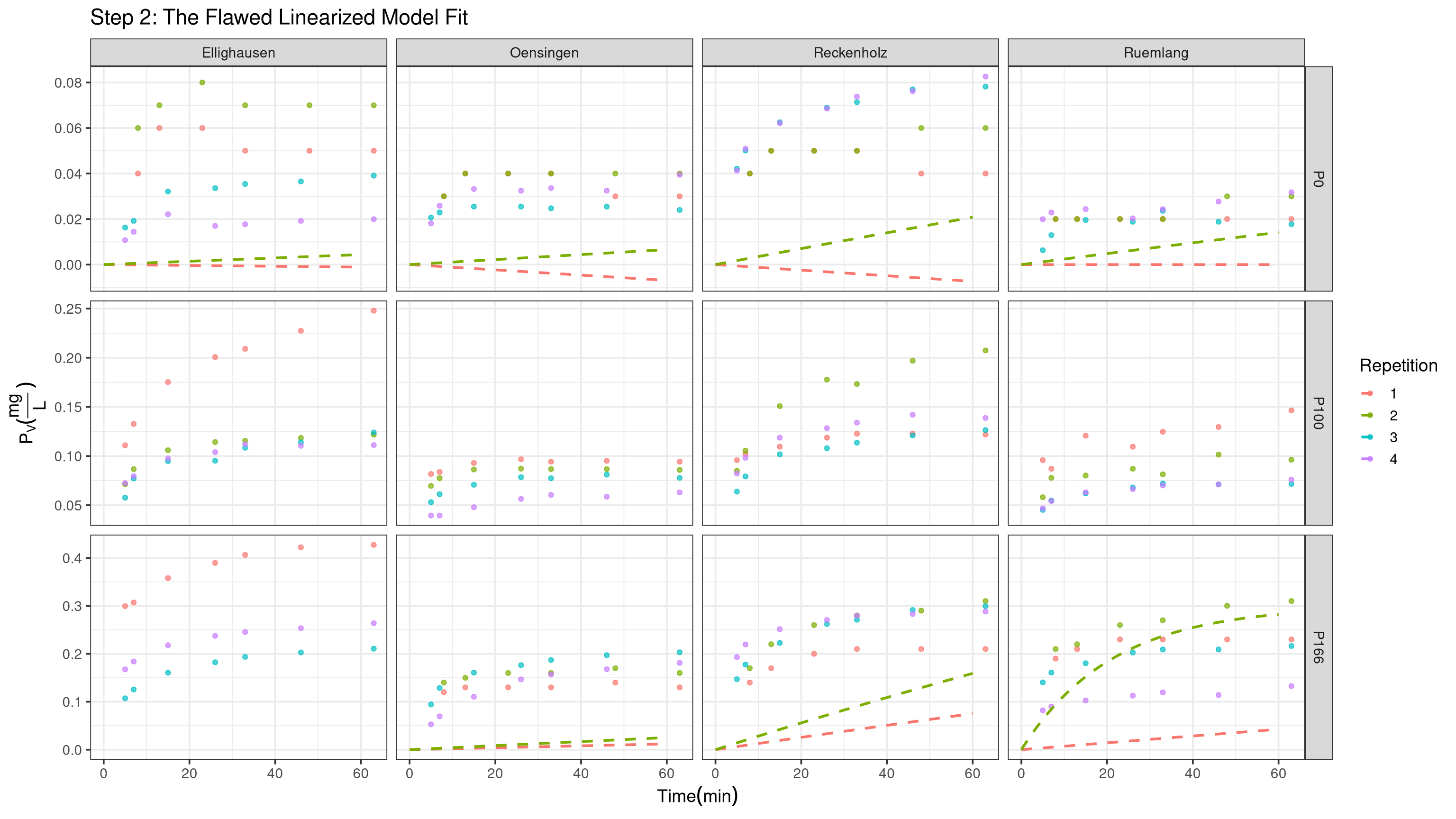
#| echo: false#| message: false#| warning: false#| fig-height: 9#| fig-width: 16p_base +geom_line(data = pred_data_flawed, aes(x = t.dt, y = pred_Pv_flawed, color = Repetition), linetype ="dashed", size =1) +labs(title ="Step 2: The Flawed Linearized Model Fit")
Method Validation
In [7]:
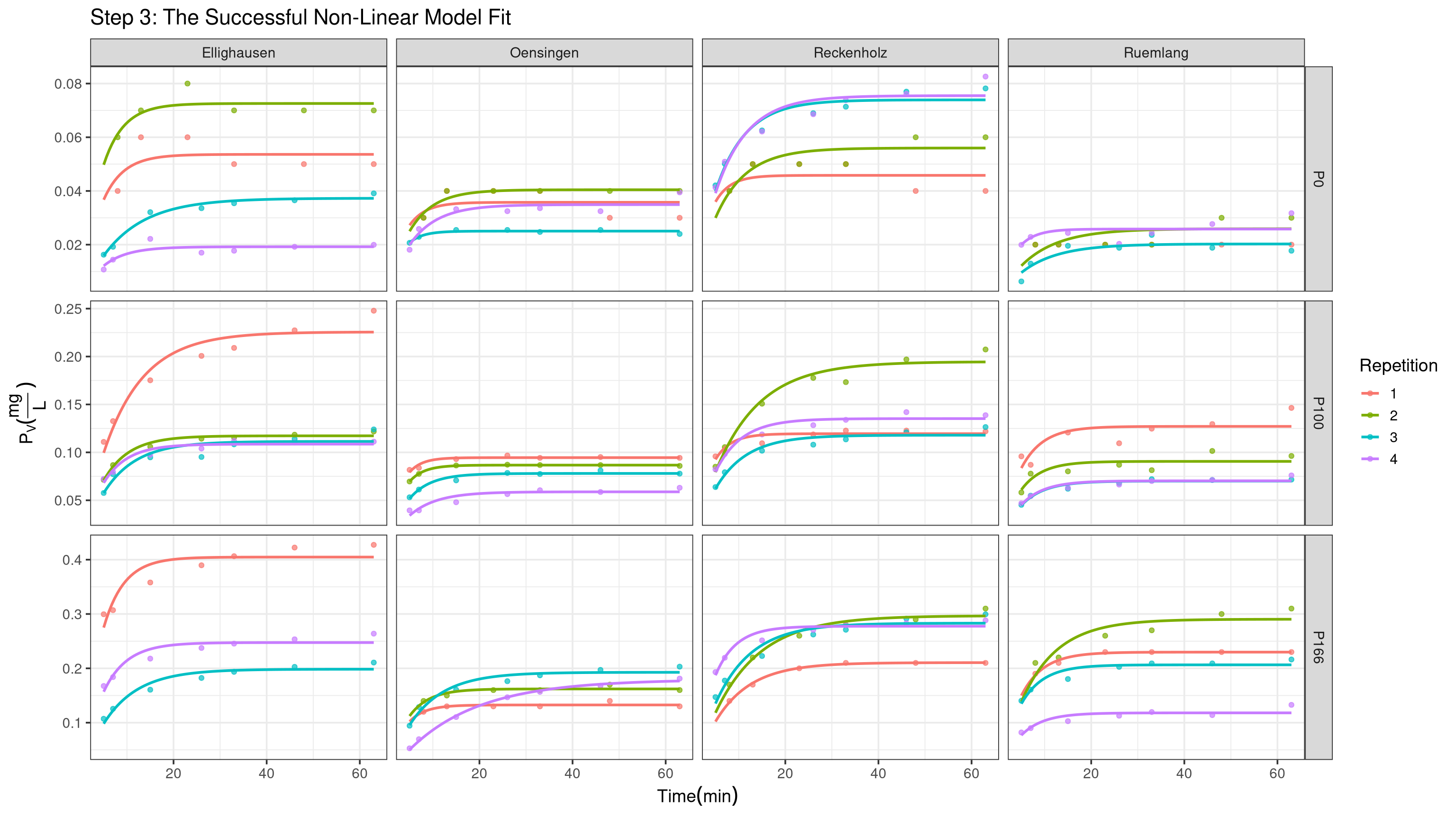
#| echo: false#| message: false#| warning: false#| fig-height: 9#| fig-width: 16p_base +geom_line(data = pred_data, aes(x = t.dt, y = pred_Pv, color = Repetition), size =1) +labs(title ="Step 3: The Successful Non-Linear Model Fit")
Method Validation
In [8]:
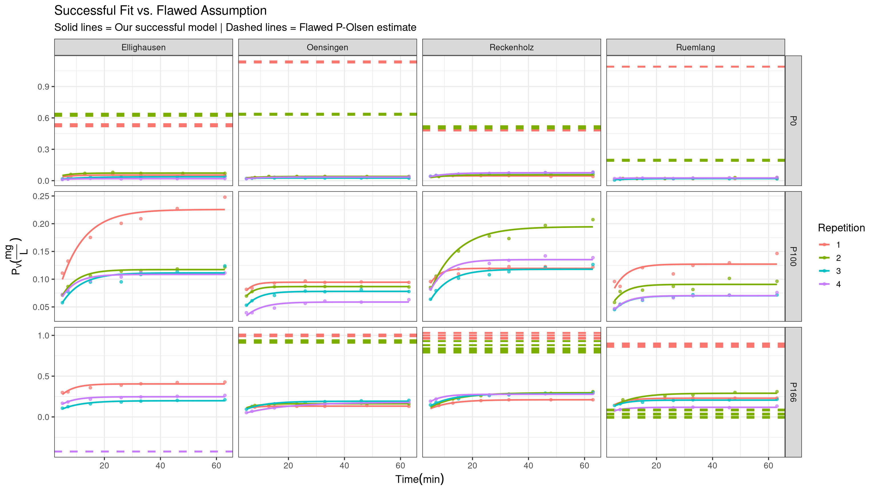
#| echo: false#| message: false#| warning: false#| fig-height: 9#| fig-width: 16# Create the data for the hlinehline_data_comparison <- d_plot %>%select(Site, Treatment, Repetition, Pv_Olsen.mg.L., Pv_labile.mg.L.) %>%mutate(flawed_estimate = Pv_Olsen.mg.L. - Pv_labile.mg.L.) %>%distinct()# Create the final comparison plotp_base +# Plot 1: Our successful non-linear model fitgeom_line(data = pred_data, aes(x = t.dt, y = pred_Pv, col = Repetition), size =1) +# Plot 2: The flawed P-Olsen - P-labile estimategeom_hline(data = hline_data_comparison,aes(yintercept = flawed_estimate, color = Repetition),linetype ="dashed", size =1.2 ) +labs(title ="Successful Fit vs. Flawed Assumption",subtitle ="Solid lines = Our successful model | Dashed lines = Flawed P-Olsen estimate" )
The Competing Predictors
We compared two approaches to predict agronomic outcomes:
The Standard Method
\(P_{CO2}\)
\(P_{AAE10}\)
These are static “snapshots” of the soil’s P capacity.
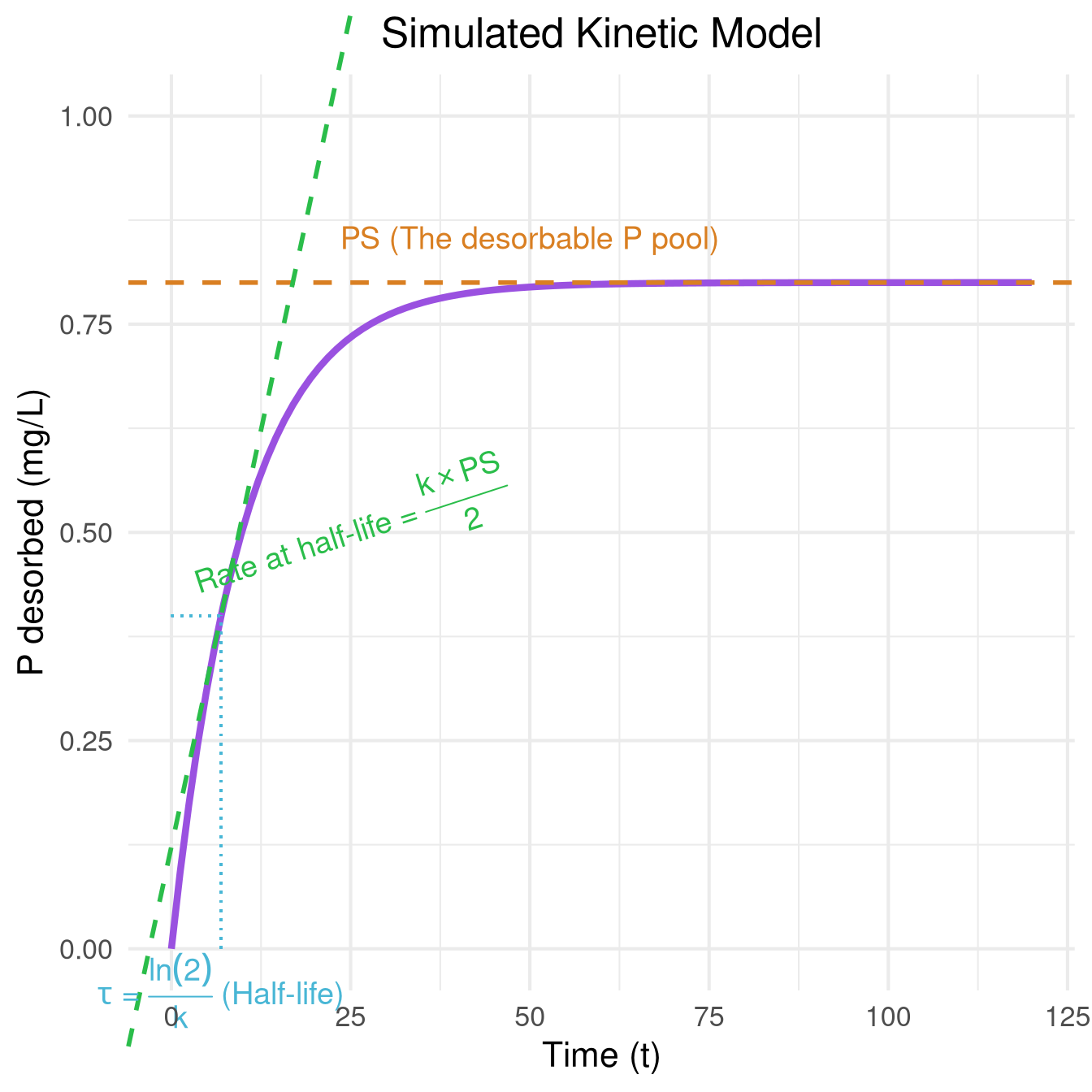
The Kinetic Method
PS (\(P^S\)): The size of the available P pool.
k: The rate of P release.
\(J_0=k*P^S\) The maximal desorption speed/initial Flow
This approach measures P as a dynamic process.
Measuring Success: The Key Outcomes
We tested the models against three agronomic metrics:
1. Normalized Yield (\(Y_{norm}\)) - How well did the crop perform relative to its maximum potential at that specific site?
2. P-Export (\(P_{up}\)) - How much phosphorus did the crop remove from the field?
3. P-Balance (\(P_{bal}\)) - What is the long-term surplus or deficit of P in the soil? This is a key indicator of sustainability.
How We Compared the Models
To ensure a fair and robust comparison, we used a consistent statistical approach:
1. Linear Mixed-Effects Models (lmer) - We built a separate model for each agronomic outcome (Yield, P-Export, P-Balance). - This approach accounts for the nested structure of the STYCS experiment (sites, years, blocks).
2. Standardized Coefficients (β) - All numeric variables were scaled and centered (mean=0, sd=1). - This allows us to directly compare the effect size of each predictor. A larger coefficient means a stronger effect.
3. The Comparison - In the following tables, each column represents a separate model where we test a different set of predictors.
What Do the P Metrics Actually Measure?
A robust P metric should reflect both the soil’s inherent properties (like texture and pH) and the impact of management (fertilization). We modeled each metric to see what drives it.
First, we tested which P metric was best at predicting site-normalized yield (\(Y_{norm}\)).
In [10]:
#| echo: false#| message: false#| warning: false# Define the models for this comparisonlmer_models_yield <-list("P_CO2"= fit.grud.CO2.Ynorm,"P_AAE10"= fit.grud.AAE10.Ynorm,"GRUD"= fit.grud.CO2.AAE10.Ynorm,"Kinetic"= fit.kin.Ynorm)# Define the clean labels for the tablecovariate_labels <-c("(Intercept)"="Intercept","log(soil_0_20_P_CO2)"="P-CO2","log(soil_0_20_P_AAE10)"="P-AAE10","k"="k","log(PS)"="PS","k:log(PS)"="J0","log(soil_0_20_P_CO2):log(soil_0_20_P_AAE10)"="P-CO2 * P-AAE10","R2m"="marginal R²","R2c"="conditional R²")model_labels_yield <-c("GRUD"="GRUD Model","Kinetic"="Kinetic Model","P_CO2"="P-CO2 only","P_AAE10"="P-AAE10 only")# Create and filter the tableresults_table_yield <-create_coef_table( lmer_models_yield,covariate_labels = covariate_labels,model_labels = model_labels_yield)results_table_yield <- results_table_yield[-1, ] # Remove intercept# Display the tablecoef_table_yield_highlighted <-highlight_significant_cells(results_table_yield)kable(coef_table_yield_highlighted,escape =FALSE, format ="html", row.names =FALSE,format.args =list(math_method ="mathjax")) %>%kable_styling(full_width =FALSE, position ="left")
Model
P-CO2 only
P-AAE10 only
GRUD Model
Kinetic Model
k
0.166
J0
-0.012
PS
0.066
P-AAE10
0.067*
0.432**
P-CO2
0.027
-0.128
P-CO2 * P-AAE10
0.149*
marginal R²
0.012
0.084
0.291
0.019
conditional R²
0.083
0.361
0.436
0.045
Predicting P-Export: A mixed Picture
In [11]:
#| label: create-p-export-table-image#| echo: false#| message: false#| warning: false# Define models and labels# ... (use the same covariate_labels and model_labels as before) ...lmer_models_export <-list("P_CO2"= fit.CO2.Pexport,"P_AAE10"= fit.AAE10.Pexport,"GRUD"= fit.grud.Pexport,"Kinetic"= fit.kin.Pexport)# Create, filter, and highlight the tableresults_table_export <-create_coef_table(lmer_models_export, covariate_labels = covariate_labels, model_labels = model_labels_yield)results_table_export <- results_table_export[-1, ]coef_table_export_highlighted <-highlight_significant_cells(results_table_export)# Build the kable objectkable(coef_table_export_highlighted,escape =FALSE, format ="html",row.names =FALSE,format.args =list(math_method ="mathjax")) %>%kable_styling(full_width =FALSE, font_size =18)
Model
P-CO2 only
P-AAE10 only
GRUD Model
Kinetic Model
k
-0.014
J0
0.080
PS
-0.018
P-AAE10
0.025
-0.015
P-CO2
0.087
0.131
P-CO2 * P-AAE10
0.011
marginal R²
0.012
0.001
0.016
0.004
conditional R²
0.654
0.685
0.796
0.789
#| label: create-p-export-table-image#| echo: false#| message: false#| warning: false# Save the kable object as a PNG image
Observation: Here, the results are less clear. P-Export is a more complex variable to predict, and no single model or predictor stands out as being consistently powerful. ## P-balance model summary:
Predicting P-Balance: The Kinetic Model is Superior